
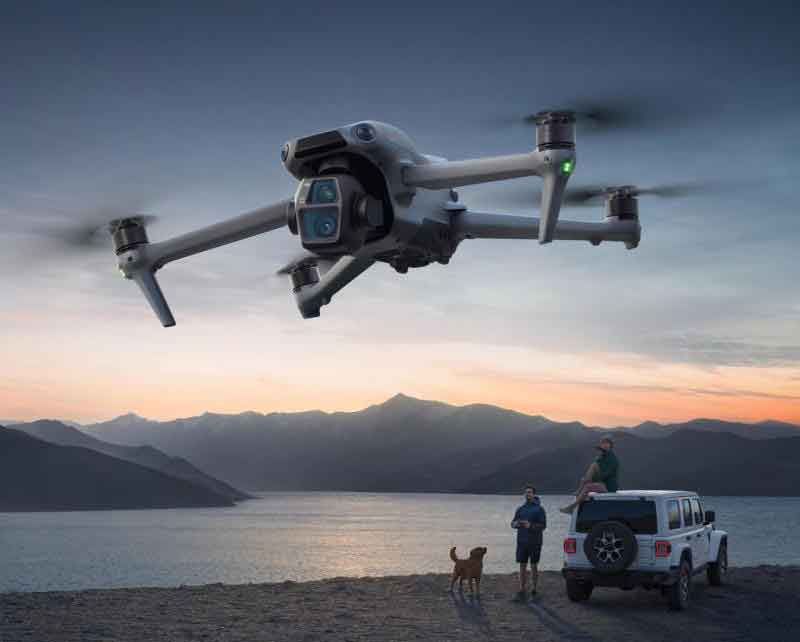
The advancement of Unmanned Aerial Vehicle (UAV) technology has revolutionized numerous fields, from logistics and agriculture to surveillance and disaster response. A critical component enabling the autonomous operation of these UAV drones is intelligent path planning. The primary objective is to compute an optimal or near-optimal flight trajectory from a start point to a destination while adhering to a complex set of constraints, including obstacle avoidance, altitude limits, and kinematic smoothness, all to ensure mission safety and efficiency. Traditional planning methods, such as A* or artificial potential fields, often struggle with dynamic environments and complex, multi-modal optimization landscapes. Similarly, while promising, methods based on reinforcement learning can require extensive training and may lack generalization. Consequently, bio-inspired metaheuristic algorithms have gained prominence for their robustness and flexibility in solving such complex, constrained optimization problems. Among these, the Marine Predator Algorithm (MPA) has shown notable performance due to its unique simulation of ocean predator-prey interactions. However, like many population-based optimizers, the standard MPA can suffer from premature convergence, imbalanced exploration-exploitation, and suboptimal performance in highly constrained search spaces like UAV drone path planning.
This paper introduces a Multi-Strategy Improved Marine Predator Algorithm (MSIMPA) specifically designed to address these shortcomings for UAV path planning. The core innovation lies in the synergistic integration of five distinct strategies into the MPA framework. We begin by formalizing a comprehensive UAV drone path planning model with a multi-objective cost function. Subsequently, we detail the enhancements: chaotic mapping for superior population initialization, an adaptive parameter adjustment mechanism for dynamic search balance, an improved differential mutation strategy for accelerated convergence, a symbiotic organism search (SOS) mechanism for enhanced local exploitation, and a neighborhood perturbation strategy to escape local optima. The efficacy of the proposed MSIMPA is rigorously validated first on a suite of CEC2017 benchmark functions, demonstrating its superior optimization capability. Finally, extensive simulation experiments for UAV drone path planning in two distinct 3D environments with multiple threats are conducted. Comparative results against the standard MPA, Grey Wolf Optimizer (GWO), Sparrow Search Algorithm (SSA), Spider Wasp Optimizer (SWO), and a Reinforcement Learning (RL) baseline confirm that MSIMPA generates shorter, safer, and smoother flight paths, proving its effectiveness and robustness for real-world UAV navigation tasks.
UAV Drone Path Planning Model and Objective Function
Formulating an accurate mathematical model is paramount for effective UAV drone path planning. The flight path is represented as a sequence of n nodes in 3D space: P = {p1, p2, …, pn}, where p1 is the start point and pn is the target. The vector between consecutive nodes is denoted as Lij, ij+1 = pj+1 – pj. The objective is to minimize a composite cost function F that encapsulates the primary mission constraints for the UAV drone.
1. Flight Path Length
Minimizing the total flight distance is crucial for energy efficiency and mission duration. The length cost F1 is the sum of Euclidean distances between all consecutive path nodes:
$$F_1 = \sum_{j=1}^{n-1} \| \mathbf{L}_{i_j, i_{j+1}} \| $$
2. Flight Safety (Obstacle Avoidance)
The UAV drone must avoid NKU known threats, each modeled as a cylinder with center OK = (xK, yK, zK) and radius RK. Let DK be the shortest distance from a path segment Lij, ij+1 to the threat’s central axis, S be a mandatory safety margin, and D be the physical radius of the UAV drone. The threat cost G for a segment relative to a single threat is defined as a piecewise function:
$$
G(\mathbf{L}_{i_j, i_{j+1}}) =
\begin{cases}
0, & D_K > R_K + S + D \\
\frac{(R_K + S + D) – D_K}{S}, & R_K + D < D_K \leq R_K + S + D \\
\infty, & D_K \leq R_K + D
\end{cases}
$$
The total safety cost F2 is the summation over all path segments and all threats:
$$F_2 = \sum_{j=1}^{n-1} \sum_{K=1}^{N_{KU}} G(\mathbf{L}_{i_j, i_{j+1}})$$
3. Flight Altitude Constraint
The UAV drone must operate within a permissible altitude band defined by a minimum Hmin and maximum Hmax above ground level. The altitude cost F3 for a path with node altitudes Hij is:
$$
F_3 = \begin{cases}
\frac{H_{max} + H_{min}}{2}, & H_{min} \leq H_{i_j} \leq H_{max} \\
\infty, & \text{otherwise}
\end{cases}
$$
4. Flight Smoothness
Abrupt turns and steep climbs increase energy consumption and induce mechanical stress. Smoothness is measured by the turning angle β between consecutive path segments and the change in climb angle θ.
Turning Angle: For three consecutive nodes pj, pj+1, pj+2, the turning angle βij is:
$$\beta_{i_j} = \arctan\left( \frac{\| \mathbf{L}_{i_j, i_{j+1}} \times \mathbf{L}_{i_{j+1}, i_{j+2}} \|}{\mathbf{L}_{i_j, i_{j+1}} \cdot \mathbf{L}_{i_{j+1}, i_{j+2}}} \right)$$
Climb Angle: The climb angle θij, ij+1 from node pj to pj+1 is:
$$\theta_{i_j, i_{j+1}} = \arctan\left( \frac{z_{i_{j+1}} – z_{i_j}}{\| \mathbf{L}_{i_j, i_{j+1}} \|} \right)$$
The total smoothness cost F4 penalizes large turning angles and sudden changes in climb angle:
$$F_4 = \alpha_1 \sum_{j=1}^{n-2} \beta_{i_j} + \alpha_2 \sum_{j=1}^{n-1} |\theta_{i_j, i_{j+1}} – \theta_{i_{j-1}, i_j}| $$
where α1 and α2 are weighting coefficients.
5. Composite Objective Function
The overall cost function for the UAV drone path planning optimization is a weighted sum of the four components:
$$F = \lambda_1 F_1 + \lambda_2 F_2 + \lambda_3 F_3 + \lambda_4 F_4$$
where λ1, λ2, λ3, λ4 are positive weights that prioritize different aspects of the flight. The optimization algorithm’s goal is to find a path P that minimizes F.
Standard Marine Predator Algorithm (MPA)
The Marine Predator Algorithm is a population-based metaheuristic inspired by the foraging behavior of ocean predators like Lévy and Brownian motions. The population, representing possible solutions (prey), is updated in three distinct phases based on a velocity ratio between predator and prey.
1. Initialization
The initial population of N prey (solutions) is randomly generated within the search space bounds [Xmin, Xmax]:
$$\mathbf{X}^0 = \mathbf{X}_{min} + \text{rand}() \cdot (\mathbf{X}_{max} – \mathbf{X}_{min})$$
An Elite matrix E is constructed by replicating the best solution (the top predator) N times. A Prey matrix P holds the current positions of all individuals.
$$\mathbf{E} =
\begin{bmatrix}
\mathbf{X}^I_{1,1} & \mathbf{X}^I_{1,2} & \dots & \mathbf{X}^I_{1,d} \\
\mathbf{X}^I_{2,1} & \mathbf{X}^I_{2,2} & \dots & \mathbf{X}^I_{2,d} \\
\vdots & \vdots & \ddots & \vdots \\
\mathbf{X}^I_{N,1} & \mathbf{X}^I_{N,2} & \dots & \mathbf{X}^I_{N,d}
\end{bmatrix},
\quad
\mathbf{P} =
\begin{bmatrix}
\mathbf{X}_{1,1} & \mathbf{X}_{1,2} & \dots & \mathbf{X}_{1,d} \\
\mathbf{X}_{2,1} & \mathbf{X}_{2,2} & \dots & \mathbf{X}_{2,d} \\
\vdots & \vdots & \ddots & \vdots \\
\mathbf{X}_{N,1} & \mathbf{X}_{N,2} & \dots & \mathbf{X}_{N,d}
\end{bmatrix}$$
2. Optimization Phases
Let T and Tmax be the current and maximum iteration number.
Phase 1: High Velocity Ratio (T ≤ Tmax/3) – Exploration: Prey moves faster than the predator. The update rule simulates Brownian motion.
$$
\begin{aligned}
\mathbf{s}_i &= \mathbf{r}_b \otimes (\mathbf{E}_i – \mathbf{r}_b \otimes \mathbf{P}_i), \quad i=1,…,N \\
\mathbf{P}_i &= \mathbf{P}_i + y \cdot \mathbf{R} \otimes \mathbf{s}_i, \quad i=1,…,N
\end{aligned}
$$
where rb is a vector of random numbers from a normal distribution (Brownian), R is a vector of uniform randoms in [0,1], ⊗ denotes element-wise multiplication, and y=0.5 is a constant.
Phase 2: Unit Velocity Ratio (Tmax/3 < T ≤ 2Tmax/3) – Transition: Speeds are comparable. The population is divided for balanced search. The first half uses Lévy flight for exploration:
$$
\begin{aligned}
\mathbf{s}_i &= \mathbf{r}_l \otimes (\mathbf{E}_i – \mathbf{r}_l \otimes \mathbf{P}_i), \quad i=1,…,N/2 \\
\mathbf{P}_i &= \mathbf{P}_i + y \cdot \mathbf{R} \otimes \mathbf{s}_i, \quad i=1,…,N/2
\end{aligned}
$$
The second half emphasizes exploitation with an adaptive step controlled by parameter C:
$$
\begin{aligned}
\mathbf{s}_i &= \mathbf{r}_b \otimes (\mathbf{r}_b \otimes \mathbf{E}_i – \mathbf{P}_i), \quad i=N/2,…,N \\
\mathbf{P}_i &= \mathbf{P}_i + C \cdot y \cdot \mathbf{s}_i, \quad i=N/2,…,N
\end{aligned}
$$
where rl is a vector based on Lévy distribution, and C is an adaptive parameter:
$$C = \left(1 – \frac{T}{T_{max}}\right)^{2T/T_{max}}$$
Phase 3: Low Velocity Ratio (T > 2Tmax/3) – Exploitation: Predator moves faster than prey, focusing on local search.
$$
\begin{aligned}
\mathbf{s}_i &= \mathbf{r}_l \otimes (\mathbf{r}_l \otimes \mathbf{E}_i – \mathbf{P}_i), \quad i=1,…,N \\
\mathbf{P}_i &= \mathbf{E}_i + C \cdot \mathbf{s}_i, \quad i=1,…,N
\end{aligned}
$$
3. Fish Aggregating Devices (FADs) Effect
To avoid local optima, the FADs effect introduces long jumps, mimicking predator behavior around fish aggregating devices.
$$\mathbf{P}_i = \begin{cases}
\mathbf{P}_i + C \cdot [\mathbf{X}_{min} + \mathbf{r} \otimes (\mathbf{X}_{max} – \mathbf{X}_{min})] \otimes \mathbf{U}, & r \leq F_A \\
\mathbf{P}_i + [F_A(1-r) + r](\mathbf{P}_{r1} – \mathbf{P}_{r2}), & r > F_A
\end{cases}$$
where FA=0.2 is the probability of FADs effect, U is a binary vector, r is a uniform random in [0,1], and r1, r2 are random prey indices.
Multi-Strategy Improved Marine Predator Algorithm (MSIMPA)
To enhance MPA’s performance for the complex UAV drone path planning problem, five strategic improvements are proposed.
1. Chaotic Mapping for Population Initialization
Replacing random initialization with a Tent-Logistic chaotic map increases initial population diversity and coverage of the search space, leading to better global exploration potential for the UAV drone path solutions.
$$x_{i+1} = \begin{cases}
\frac{bx_i(4(1-x_i))}{2} + \frac{(4-b)x_i}{2}, & 0 \leq x_i \leq 0.5 \\
\frac{b(1-x_i)(4x_i-1)}{2} + \frac{(4-b)(1-x_i)}{2}, & 0.5 < x_i \leq 1
\end{cases}$$
where xi ∈ (0,1) is the chaotic variable, and b is a control parameter. The initial prey position is then: X0 = Xmin + x ⊗ (Xmax – Xmin).
2. Adaptive Parameter Adjustment Strategy
The parameter C crucially balances exploration and exploitation. We introduce a non-linear inertia weight ω to dynamically adjust it, improving convergence behavior throughout the UAV drone path search.
$$\omega = \mu \times e^{\left[-\left( \frac{T}{T_{max}} \right)^{\mu} \right]}$$
where μ is a control parameter (typically 1-3). The adaptive parameter C is then modified as:
$$C = \omega \times 2 \times (T / T_{max})$$
This allows for a more sensitive and dynamic tuning of the step size during different phases of the UAV drone optimization process.
3. Improved Differential Mutation Strategy
In the initial high-velocity phase, we integrate a differential evolution-inspired mutation with Lévy flight to accelerate global exploration and improve the quality of initial paths for the UAV drone.
$$
\begin{aligned}
\mathbf{s}_i &= \mathbf{r}_l \otimes (\mathbf{P}_{r3} – \mathbf{P}_{r4}) + \mathbf{r}_l \otimes (\mathbf{P}_{r1} – \mathbf{P}_{r2}), \quad i=1,…,N \\
\mathbf{P}_i &= \mathbf{E}_i + C \cdot \mathbf{s}_i, \quad i=1,…,N
\end{aligned}
$$
where r1, r2, r3, r4 are distinct random indices. This strategy enhances information sharing among individuals, fostering a more effective search direction.
4. Symbiotic Organism Search (SOS) Mechanism
During the low-velocity exploitation phase, we embed the mutualism phase from the SOS algorithm. This simulates a mutually beneficial relationship between two organisms (solutions), refining the UAV drone path locally around the current best solution.
$$
\begin{aligned}
\mathbf{M} &= \frac{\mathbf{P}_i^t + \mathbf{P}_j^t}{2} + \text{rand}(0,1) \\
\mathbf{P}_i^{t+1} &= \mathbf{P}_i^t + \text{rand}(0,1) \times (\mathbf{P}_{\text{best}}^t – \mathbf{M} \times O_1) \\
\mathbf{P}_j^{t+1} &= \mathbf{P}_j^t + \text{rand}(0,1) \times (\mathbf{P}_{\text{best}}^t – \mathbf{M} \times O_2)
\end{aligned}
$$
where Pjt is a randomly selected partner organism, Pbestt is the current elite (best predator), and O1, O2 ∈ [1,2] are mutual benefit factors. This mechanism intensifies local search around promising regions.
5. Neighborhood Perturbation Strategy
To prevent premature stagnation, a neighborhood perturbation is applied to the best solution after updates. It creates a candidate solution in the vicinity of the current best UAV drone path.
$$x_{\text{best},j}(t+1) = \begin{cases}
0.5 \times (x_{\text{best},j}(t) – r_5), & r_5 < 0.5 \\
x_{\text{best},j}(t) + 0.5 \times r_5, & r_5 \geq 0.5
\end{cases}$$
where xbest,j(t) is the j-th dimension of the best solution, and r5 ∈ [0,1]. A greedy selection is then performed:
$$
\mathbf{X}_{\text{best}}^{\text{new}} = \begin{cases}
\mathbf{X}_{\text{candidate}}, & f(\mathbf{X}_{\text{candidate}}) < f(\mathbf{X}_{\text{best}}^{\text{old}}) \\
\mathbf{X}_{\text{best}}^{\text{old}}, & \text{otherwise}
\end{cases}
$$
This ensures the population’s leader only improves, maintaining search progress.
Algorithm Performance Validation on Benchmark Functions
Before applying MSIMPA to UAV drone path planning, its core optimization capability is tested on the CEC2017 benchmark suite. Functions F1 (unimodal), F3, F4, F5 (multimodal), and F10, F11 (hybrid composition) are selected. The search space is [-100, 100]D (D=30). Parameters: Population N=50, Max Iterations Tmax=500. Each algorithm runs 30 times independently. The results, comparing MSIMPA against standard MPA, SSA, and GWO, are summarized below.
| Function | Type | MSIMPA | MPA | SSA | GWO |
|---|---|---|---|---|---|
| F1 | Unimodal | 1.00E+02 ± 6.70E-06 | 2.42E+02 ± 3.56E+03 | 2.31E+02 ± 3.12E+03 | 2.62E+02 ± 4.11E+02 |
| F3 | Multimodal | 3.11E+02 ± 1.11E-03 | 3.95E+02 ± 1.48E+02 | 4.22E+02 ± 2.47E+03 | 3.89E+02 ± 1.27E+02 |
| F4 | Multimodal | 4.03E+02 ± 1.67E-07 | 5.11E+02 ± 6.31E+03 | 6.05E+02 ± 4.22E+05 | 4.89E+02 ± 2.87E+02 |
| F5 | Multimodal | 5.86E+02 ± 1.12E+02 | 8.86E+02 ± 2.12E+05 | 7.55E+02 ± 1.02E+05 | 9.12E+02 ± 4.32E+05 |
| F10 | Hybrid | 1.21E+03 ± 5.22E+02 | 2.15E+04 ± 1.88E+07 | 8.81E+03 ± 7.56E+05 | 4.31E+03 ± 5.43E+05 |
| F11 | Hybrid | 2.01E+03 ± 1.08E+02 | 4.53E+03 ± 2.31E+07 | 3.08E+03 ± 5.08E+05 | 3.45E+03 ± 6.01E+04 |
The results clearly demonstrate MSIMPA’s superiority. It achieves the lowest mean error and remarkably small standard deviation across all function types. This indicates not only superior accuracy in finding the global optimum but also exceptional stability and robustness—critical attributes for reliable UAV drone path planning where consistent performance is required.
UAV Drone Path Planning Experiments and Results
To evaluate the practical efficacy of MSIMPA, we conduct UAV drone path planning simulations in two distinct 3D environments with multiple cylindrical threat zones. The algorithms are tasked with minimizing the composite cost function F. The parameters for the simulations are as follows:
| Parameter | Value |
|---|---|
| UAV Drone Operational Speed | 0 – 25 m/s |
| UAV Drone Flight Altitude Range | 50 – 300 m |
| Max Turn Angle | 45° |
| Max Climb/Dive Angle | 45° |
| UAV Drone Physical Radius (D) | 2 m |
| Safety Margin (S) | 10 m |
| Objective Weights (λ1, λ2, λ3, λ4) | 0.4, 0.3, 0.2, 0.1 |
| Algorithm Population Size (N) | 50 |
| Max Iterations (Tmax) | 200 |
| Map | Start Point (x,y,z) m | Target Point (x,y,z) m | Threats (Center [x,y,z], Radius R) m |
|---|---|---|---|
| Map 1 | (200, 100, 50) | (900, 700, 150) | Th1: ([400, 500, 200], 50) Th2: ([600, 200, 200], 40) Th3: ([500, 350, 200], 50) Th4: ([800, 650, 200], 70) |
| Map 2 | (200, 100, 50) | (900, 700, 150) | Th1: ([400, 300, 200], 50) Th2: ([500, 220, 200], 40) Th3: ([500, 350, 200], 50) Th4: ([700, 500, 200], 30) Th5: ([800, 650, 200], 70) Th6: ([650, 750, 150], 50) |
Results Analysis for Map 1
In Map 1, MSIMPA successfully generates a smooth and efficient path for the UAV drone. The 3D trajectory and top-down view illustrate that MSIMPA’s path navigates the threat zones with ample clearance, maintaining a relatively direct course. In contrast, paths from SSA and SWO show noticeable detours and sharper turns. The RL baseline generates a feasible but suboptimal path with unnecessary maneuvering. The convergence curve plot clearly shows MSIMPA’s advantage: it starts with a better initial solution (due to chaotic initialization) and converges faster to a lower final cost than MPA, GWO, SSA, SWO, and RL. This indicates its enhanced exploration and exploitation balance.
Results Analysis for Map 2
Map 2 presents a more cluttered environment with six threats, posing a greater challenge. MSIMPA again demonstrates robust performance, finding a path that elegantly weaves between obstacles. Notably, paths from MPA, GWO, and SSA exhibit more pronounced zig-zagging near the dense threat cluster in the central-right area, indicating difficulty in fine-tuning the path. SWO’s path shows an extremely sharp, almost right-angled turn, which is kinematically infeasible for a typical UAV drone. MSIMPA’s convergence is the most rapid and stable, reaching the lowest cost value, which translates to a shorter, safer, and smoother path.
| Algorithm | Map 1 Flight Distance (km) | Map 2 Flight Distance (km) |
|---|---|---|
| MSIMPA (Proposed) | 11.67 | 11.38 |
| MPA | 12.04 | 12.54 |
| GWO | 12.44 | 12.43 |
| SSA | 13.41 | 11.68 |
| SWO | 14.61 | 15.17 |
| RL | 13.74 | 12.55 |
The quantitative results in Table 4 unequivocally confirm MSIMPA’s superiority. In both test environments, the flight distance calculated by MSIMPA is the shortest among all compared algorithms. For instance, in Map 1, MSIMPA’s path is 0.37 km shorter than standard MPA, 0.77 km shorter than GWO, and significantly shorter than SWO and RL. This directly translates to lower energy consumption and faster mission completion time for the autonomous UAV drone.
Conclusion
This paper presented a novel Multi-Strategy Improved Marine Predator Algorithm (MSIMPA) for solving the complex, constrained optimization problem of UAV drone path planning. The proposed enhancements—chaotic initialization, adaptive parameter tuning, differential mutation, symbiotic search, and neighborhood perturbation—were meticulously designed to address the inherent limitations of the standard MPA, specifically its tendency for premature convergence and suboptimal exploration-exploitation balance. The integration of these strategies resulted in an algorithm with significantly improved population diversity, convergence speed, and the ability to escape local optima.
Rigorous testing on the CEC2017 benchmark suite first established the superior optimization performance of MSIMPA over standard MPA and other state-of-the-art algorithms. Subsequent application to 3D UAV drone path planning in environments with multiple threats provided compelling practical validation. The simulation results demonstrated that MSIMPA consistently generates flight paths that are shorter, adhere more strictly to safety constraints, and are smoother compared to those generated by MPA, GWO, SSA, SWO, and an RL baseline. The shorter flight distance directly implies enhanced operational efficiency for the UAV drone in terms of energy savings and mission time. Therefore, MSIMPA proves to be a highly effective and reliable metaheuristic solver for autonomous UAV drone navigation tasks, offering a robust solution for real-world path planning challenges.