
In my work, I focus on reliable wireless links for UAV drones because UAV drones are becoming active nodes in 5G and beyond-5G networks. UAV drones can serve as aerial base stations, aerial terminals, and aerial relays, but their mobility and the complexity of the propagation environment make the wireless channel time-varying, spatially correlated, and sometimes blocked. I therefore study two tightly connected problems: MIMO channel estimation for UAV drones and beam tracking for UAV drones in millimeter-wave links assisted by a reconfigurable intelligent surface. My objective is to reduce estimation error, control pilot overhead, and improve tracking accuracy when UAV drones move.
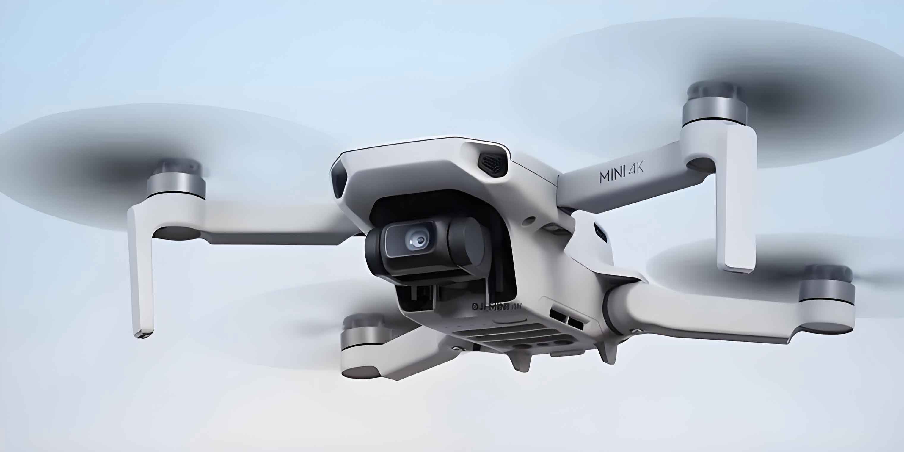
The first part of my study considers a downlink MIMO communication link between an aerial base station and a ground terminal. The channel is not assumed to be independent and identically distributed. This matters because UAV drones often experience line-of-sight, strong directional components, shadowing, and Doppler effects. Traditional least-squares, minimum mean-square-error, and linear minimum mean-square-error estimators can work well in simple cases, but their performance degrades when the channel changes quickly and when the pilot budget is limited. I propose a Kalman-filter-based MIMO channel estimator that uses a specific sparse pilot pattern. The sparse pattern balances pilot overhead, estimator convergence, and beamforming quality. The receiver feeds channel state information back to the UAV drone transmitter, and the transmitter uses the feedback for precoding and beamforming. My simulation results show that the Kalman-filter estimator has lower mean-square error than the traditional least-squares estimator under the same conditions.
The second part of my study considers RIS-assisted beam tracking for UAV drones. A reconfigurable intelligent surface can reshape the propagation environment by tuning the phase shifts of its reflecting elements. Because the RIS can create an additional controllable path, it is attractive when the direct path to a UAV drone is blocked. I use an extended Kalman filter because the measurement model is nonlinear with respect to angle of departure, angle of arrival, and complex channel gain. The state evolves with a Gaussian-Markov model, and the EKF linearizes the measurement function through a Jacobian. My simulations compare RIS-assisted tracking with tracking without a RIS. The RIS-assisted extended Kalman filter achieves lower tracking error for UAV drones, especially when the signal-to-noise ratio is moderate or high.
I organize the technical discussion around several foundations: wireless channel fading, MIMO and OFDM transmission, pilot design, Kalman filtering, autoregressive modeling, millimeter-wave propagation, and RIS phase control. I use tables and equations to summarize the main relationships because UAV drones require both mathematical clarity and practical design rules. In particular, I emphasize that the choice of pilot pattern, antenna count, Doppler frequency, and coherence time directly affects the accuracy of channel estimation and beam tracking for UAV drones.
$$y(t)=x(t)+n(t)$$
The above additive noise model is the simplest starting point. In a real UAV drones link, the received signal is also shaped by path loss, shadowing, multipath, and Doppler spread. Large-scale fading changes slowly over distance, while small-scale fading changes over fractions of a wavelength. For UAV drones, the relative motion between transmitter and receiver can be significant, so the Doppler effect cannot be ignored. I therefore begin with the standard fading decomposition and then connect it to MIMO channel estimation.
Large-scale fading includes path loss and shadowing. The free-space received power can be written as follows.
$$P_r(d)=\frac{P_t G_t G_r \lambda^2}{(4\pi d)^2 L}$$
Here, \(P_t\) is the transmit power, \(G_t\) and \(G_r\) are antenna gains, \(\lambda\) is the wavelength, \(d\) is the distance, and \(L\) is the system loss. The corresponding path loss in decibels is obtained from the difference between transmit and received power.
$$PL(d)=10\log_{10}\left(\frac{P_t}{P_r(d)}\right)=10\log_{10}\left(\frac{(4\pi d)^2 L}{G_t G_r \lambda^2}\right)$$
Shadowing is often modeled as a log-normal random variation around the path loss.
$$PL(d)=PL(d_0)+10n\log_{10}\left(\frac{d}{d_0}\right)+X_\sigma$$
In this expression, \(n\) is the path-loss exponent, \(d_0\) is a reference distance, and \(X_\sigma\) is a zero-mean Gaussian random variable with standard deviation \(\sigma\). For UAV drones, the path-loss exponent depends on altitude, terrain, and whether the link is over urban, suburban, or rural areas.
Small-scale fading is caused by multipath and Doppler. The Doppler shift for a moving UAV drone is
$$f_d=\frac{v}{\lambda}\cos\theta$$
where \(v\) is the relative velocity and \(\theta\) is the angle between the direction of motion and the arrival direction. The maximum Doppler shift is \(f_m=v/\lambda\). The coherence time is approximately
$$T_c\approx \frac{1}{2f_m}$$
and the coherence bandwidth is related to the delay spread. If the signal bandwidth is smaller than the coherence bandwidth, the channel is flat; otherwise, it is frequency selective. If the symbol duration is shorter than the coherence time, the channel is fast fading; otherwise, it is slow fading. UAV drones may operate in either regime depending on speed, carrier frequency, and waveform parameters.
| Fading type | Cause | Time or frequency scale | Impact on UAV drones |
|---|---|---|---|
| Path loss | Distance and propagation medium | Large distance | Sets link budget and coverage radius |
| Shadowing | Obstacles and terrain | Slow variation | Causes temporary link degradation |
| Multipath | Reflection, diffraction, scattering | Delay spread | Creates frequency selectivity and MIMO richness |
| Doppler | Relative motion | Coherence time | Makes channel estimation and beam tracking harder |
| Flat fading | Signal bandwidth below coherence bandwidth | Frequency-flat | Simplifies equalization but not necessarily tracking |
| Frequency-selective fading | Signal bandwidth above coherence bandwidth | Frequency-dependent | Requires OFDM or equalization |
For MIMO transmission, I use the standard baseband model
$$\mathbf{y}=\mathbf{H}\mathbf{x}+\mathbf{n}$$
where \(\mathbf{y}\in\mathbb{C}^{N_r\times 1}\) is the received vector, \(\mathbf{H}\in\mathbb{C}^{N_r\times N_t}\) is the channel matrix, \(\mathbf{x}\in\mathbb{C}^{N_t\times 1}\) is the transmitted vector, and \(\mathbf{n}\in\mathbb{C}^{N_r\times 1}\) is additive white Gaussian noise. The number of transmit antennas is \(N_t\), and the number of receive antennas is \(N_r\). For UAV drones, MIMO provides spatial diversity, spatial multiplexing, and beamforming gains, but it also increases the number of unknown channel coefficients. This creates a direct conflict between estimation accuracy and pilot overhead.
The capacity of a point-to-point MIMO link with independent Rayleigh fading can be summarized as
$$C=\min(N_t,N_r)B\log_2\left(1+\frac{S}{N}\right)$$
under ideal conditions. In practice, the achievable rate depends on channel correlation, rank, feedback quality, and the accuracy of channel state information. For UAV drones, the channel may be dominated by a few strong paths, so the effective rank can be low. This sparsity can be exploited, but it also means that angle estimation and beam tracking become important.
OFDM is often combined with MIMO because it converts a frequency-selective channel into a set of parallel flat subchannels. For each subcarrier \(k\), the input-output relation is
$$\mathbf{y}[k]=\mathbf{H}[k]\mathbf{x}[k]+\mathbf{n}[k]$$
Pilot symbols are inserted in the time-frequency grid so that the receiver can estimate \(\mathbf{H}[k]\). The three classical pilot patterns are block-type, comb-type, and lattice-type. I summarize them in the following table because pilot design is central to my proposed estimator.
| Pilot pattern | Time-frequency placement | Typical use | Advantage | Limitation |
|---|---|---|---|---|
| Block type | All subcarriers in selected OFDM symbols | Slow fading | Simple and robust for slow channels | Not ideal for fast Doppler |
| Comb type | Selected subcarriers in every OFDM symbol | Fast fading | Tracks time variation | Needs frequency interpolation |
| Lattice type | Selected subcarriers and selected symbols | Doubly selective channels | Balances time and frequency sampling | More complex design |
For UAV drones, the pilot pattern must respect the coherence time and coherence bandwidth. If the UAV drone moves quickly, the pilot repetition interval must be short enough to track phase rotation. If the delay spread is large, the pilot spacing in frequency must be small enough to avoid aliasing. At the same time, too many pilots reduce spectral efficiency. My proposed design therefore uses a sparse comb-like pattern whose density is chosen according to Doppler frequency, antenna configuration, and target mean-square error.
The Kalman filter is a recursive Bayesian estimator for linear Gaussian state-space models. I use it because channel coefficients evolve in time and can be treated as a hidden state. The canonical prediction and update equations are as follows.
$$\mathbf{x}_{t|t-1}=\mathbf{A}_t\mathbf{x}_{t-1|t-1}+\mathbf{B}_t\mathbf{u}_t+\mathbf{w}_t$$
$$\mathbf{y}_t=\mathbf{C}_t\mathbf{x}_{t|t-1}+\mathbf{v}_t$$
$$\mathbf{P}_{t|t-1}=\mathbf{A}_t\mathbf{P}_{t-1|t-1}\mathbf{A}_t^H+\mathbf{Q}_t$$
$$\mathbf{K}_t=\mathbf{P}_{t|t-1}\mathbf{C}_t^H\left(\mathbf{C}_t\mathbf{P}_{t|t-1}\mathbf{C}_t^H+\mathbf{R}_t\right)^{-1}$$
$$\mathbf{x}_{t|t}=\mathbf{x}_{t|t-1}+\mathbf{K}_t\left(\mathbf{y}_t-\mathbf{C}_t\mathbf{x}_{t|t-1}\right)$$
$$\mathbf{P}_{t|t}=\left(\mathbf{I}-\mathbf{K}_t\mathbf{C}_t\right)\mathbf{P}_{t|t-1}$$
Here, \(\mathbf{x}_{t|t-1}\) is the predicted state, \(\mathbf{P}_{t|t-1}\) is the predicted covariance, \(\mathbf{K}_t\) is the Kalman gain, \(\mathbf{Q}_t\) is the process noise covariance, and \(\mathbf{R}_t\) is the measurement noise covariance. For UAV drones MIMO channel estimation, the state is the vectorized channel matrix or a low-dimensional representation of it. The measurement is formed from received pilot symbols.
When the measurement model or state model is nonlinear, I use the extended Kalman filter. The prediction and update steps become
$$\mathbf{x}_{t|t-1}=f(\mathbf{x}_{t-1|t-1},\mathbf{u}_t)$$
$$\mathbf{y}_t=h(\mathbf{x}_{t|t-1})+\mathbf{v}_t$$
$$\mathbf{P}_{t|t-1}=\mathbf{A}_t\mathbf{P}_{t-1|t-1}\mathbf{A}_t^H+\mathbf{Q}_t$$
$$\mathbf{K}_t=\mathbf{P}_{t|t-1}\mathbf{J}_t^H\left(\mathbf{J}_t\mathbf{P}_{t|t-1}\mathbf{J}_t^H+\mathbf{R}_t\right)^{-1}$$
$$\mathbf{x}_{t|t}=\mathbf{x}_{t|t-1}+\mathbf{K}_t\left(\mathbf{y}_t-h(\mathbf{x}_{t|t-1})\right)$$
$$\mathbf{P}_{t|t}=\left(\mathbf{I}-\mathbf{K}_t\mathbf{J}_t\right)\mathbf{P}_{t|t-1}$$
where \(\mathbf{A}_t\) is the Jacobian of \(f\), and \(\mathbf{J}_t\) is the Jacobian of \(h\). The EKF is suitable for beam tracking because the received signal depends on angles through array response vectors, and these dependencies are nonlinear.
| Filter | System assumption | Strength | Weakness | Typical UAV drones use |
|---|---|---|---|---|
| Kalman filter | Linear Gaussian | Optimal for linear models | Poor for strongly nonlinear models | Time-varying MIMO channel estimation |
| Extended Kalman filter | Nonlinear with local linearization | Handles angle-dependent measurements | Jacobian derivation and linearization error | RIS-assisted beam tracking |
| Unscented Kalman filter | Nonlinear with sigma points | Better robustness in some nonlinear cases | Higher complexity | Advanced tracking for UAV drones |
To model temporal correlation, I use an autoregressive process. An AR(\(p\)) model for a scalar sequence is
$$x_t=a_0+a_1x_{t-1}+a_2x_{t-2}+\cdots+a_px_{t-p}+\epsilon_t$$
where \(\epsilon_t\sim\mathcal{N}(0,\sigma^2)\). For zero-mean AR(\(p\)), the constant term is removed. In matrix form, I write the channel state evolution as
$$\mathbf{H}_t=\sum_{i=1}^{p}\mathbf{A}_i\mathbf{H}_{t-i}+\mathbf{U}_t$$
where \(\mathbf{A}_i\) are AR coefficient matrices and \(\mathbf{U}_t\) is process noise. The Yule-Walker equations provide a classical way to estimate the AR parameters:
$$\mathbf{R}_{1:p}=\mathbf{R}_{0:p-1}\begin{bmatrix}\mathbf{A}_1&\mathbf{A}_2&\cdots&\mathbf{A}_p\end{bmatrix}^T$$
$$\begin{bmatrix}\mathbf{A}_1&\mathbf{A}_2&\cdots&\mathbf{A}_p\end{bmatrix}^T=\mathbf{R}_{0:p-1}^{-1}\mathbf{R}_{1:p}$$
The covariance of the driving noise is
$$\mathbf{Q}=\mathbf{R}_0-\sum_{i=1}^{p}\mathbf{A}_i\mathbf{R}_i^H$$
In my design, I use a low-order AR model to keep complexity manageable. A first-order AR model is often sufficient when the coherence time is much longer than the symbol duration. Higher-order models can capture more memory but increase computational cost and require more training data.
Traditional channel estimation methods provide useful baselines. The least-squares estimator minimizes the squared error between the received pilot signal and the hypothesized signal.
$$\mathbf{H}_{LS}=\arg\min_{\mathbf{H}}\|\mathbf{Y}-\mathbf{X}\mathbf{H}\|_F^2$$
$$\mathbf{H}_{LS}=\left(\mathbf{X}^H\mathbf{X}\right)^{-1}\mathbf{X}^H\mathbf{Y}$$
If the pilot matrix has orthogonal columns and equal power, this simplifies to
$$\mathbf{H}_{LS}=\mathbf{X}^{-1}\mathbf{Y}$$
The mean-square error of LS is proportional to the inverse signal-to-noise ratio:
$$MSE_{LS}=\frac{\sigma_n^2}{\sigma_x^2}$$
Thus, LS is simple but sensitive to noise and ill-conditioned pilots. In deep fading, its performance can be poor.
The minimum mean-square-error estimator uses second-order statistics.
$$\mathbf{H}_{MMSE}=\mathbf{R}_{HY}\mathbf{R}_{YY}^{-1}\mathbf{Y}$$
For the model \(\mathbf{Y}=\mathbf{X}\mathbf{H}+\mathbf{Z}\), the MMSE estimator becomes
$$\mathbf{H}_{MMSE}=\mathbf{R}_{HH}\mathbf{X}^H\left(\mathbf{X}\mathbf{R}_{HH}\mathbf{X}^H+\sigma_z^2\mathbf{I}\right)^{-1}\mathbf{Y}$$
Equivalently, it can be written in terms of the LS estimate:
$$\mathbf{H}_{MMSE}=\left(\mathbf{R}_{HH}^{-1}+\mathbf{X}^H\mathbf{X}\sigma_z^{-2}\right)^{-1}\mathbf{X}^H\mathbf{Y}$$
The linear minimum mean-square-error estimator reduces complexity by replacing the instantaneous pilot covariance with its average.
$$\mathbf{H}_{LMMSE}=\mathbf{R}_{HH}\left(\mathbf{R}_{HH}+\frac{\beta}{SNR}\mathbf{I}\right)^{-1}\mathbf{H}_{LS}$$
Here, \(\beta\) depends on the modulation scheme and constellation. LMMSE has lower complexity than MMSE but still requires channel correlation knowledge.
| Estimator | Required statistics | Complexity | Noise sensitivity | Use in UAV drones MIMO |
|---|---|---|---|---|
| LS | None beyond pilots | Low | High | Baseline and initialization |
| MMSE | Channel and noise covariance | High | Low | Accurate but costly |
| LMMSE | Channel covariance and SNR | Medium | Medium | Practical compromise |
| Kalman filter | State model and noise covariance | Recursive, medium | Low when model matches | Time-varying UAV drones MIMO |
My proposed channel estimator for UAV drones MIMO is built on a sparse pilot pattern and a Kalman filter. I consider a downlink scenario where the aerial transmitter sends pilots to a ground receiver. The receiver estimates the channel, feeds back quantized or compressed channel state information, and the transmitter uses it for precoding. The pilot pattern is comb-like in frequency and periodic in time. It is designed so that the number of pilot symbols is much smaller than the number of channel coefficients, yet the Kalman filter can still track the dominant subspace. This is important for UAV drones because the channel dimension grows with \(N_tN_r\), and pilot overhead can become prohibitive if a full pilot grid is used.
I define the state vector at time \(t\) as the vectorized channel matrix:
$$\mathbf{h}_t=\operatorname{vec}(\mathbf{H}_t)$$
The state evolution is
$$\mathbf{h}_t=\mathbf{F}\mathbf{h}_{t-1}+\mathbf{w}_t$$
where \(\mathbf{F}\) is obtained from the AR model. The pilot observation is
$$\mathbf{y}_t=\mathbf{X}_t\mathbf{h}_t+\mathbf{v}_t$$
or, in matrix form,
$$\mathbf{Y}_t=\mathbf{X}_t\mathbf{H}_t+\mathbf{V}_t$$
The Kalman recursion for the MIMO channel is
$$\mathbf{h}_{t|t-1}=\mathbf{F}\mathbf{h}_{t-1|t-1}$$
$$\mathbf{P}_{t|t-1}=\mathbf{F}\mathbf{P}_{t-1|t-1}\mathbf{F}^H+\mathbf{Q}_t$$
$$\mathbf{K}_t=\mathbf{P}_{t|t-1}\mathbf{X}_t^H\left(\mathbf{X}_t\mathbf{P}_{t|t-1}\mathbf{X}_t^H+\mathbf{R}_t\right)^{-1}$$
$$\mathbf{h}_{t|t}=\mathbf{h}_{t|t-1}+\mathbf{K}_t\left(\mathbf{y}_t-\mathbf{X}_t\mathbf{h}_{t|t-1}\right)$$
$$\mathbf{P}_{t|t}=\left(\mathbf{I}-\mathbf{K}_t\mathbf{X}_t\right)\mathbf{P}_{t|t-1}$$
The initialization uses the LS estimate from the first pilot block:
$$\mathbf{H}_{0|0}=\mathbf{H}_{LS}$$
$$\mathbf{P}_{0|0}=\mathbb{E}\left[(\mathbf{H}_{0|0}-\mathbb{E}[\mathbf{H}_{0|0}])(\mathbf{H}_{0|0}-\mathbb{E}[\mathbf{H}_{0|0}])^H\right]$$
The AR coefficient matrix is estimated from channel correlation matrices. For a first-order model,
$$\mathbf{H}_t=\mathbf{A}_1\mathbf{H}_{t-1}+\mathbf{U}_t$$
and the Yule-Walker estimate is
$$\mathbf{A}_1=\mathbf{R}_1\mathbf{R}_0^{-1}$$
$$\mathbf{Q}=\mathbf{R}_0-\mathbf{A}_1\mathbf{R}_1^H$$
In my simulations, I compare the Kalman filter with LS under different Doppler frequencies and antenna configurations. The metrics are mean-square error and robustness. The following table summarizes the qualitative behavior I observe.
| Doppler frequency | Antenna configuration | LS behavior | Kalman behavior | Main reason |
|---|---|---|---|---|
| Low | 1×1 | Acceptable | Better | Temporal correlation is strong |
| Medium | 1×1 | Degrades | Clearly better | KF predicts phase and amplitude drift |
| Low | 4×4 | Moderate error | Lower error | KF reduces noise through recursion |
| High | 4×4 | Poor | Less poor | Temporal correlation weakens |
| Very high | 8×8 | Very poor with sparse pilots | Still limited | Pilot density becomes insufficient |
A key part of my contribution is the pilot density rule. If the coherence time is \(T_c\) and the pilot repetition interval in time is \(T_p\), then I require
$$T_p\le \frac{T_c}{2}$$
to avoid severe tracking loss. In frequency, if the delay spread is \(\tau_{\max}\), the coherence bandwidth is approximately \(B_c\approx 1/\tau_{\max}\), and the pilot spacing \(\Delta f_p\) should satisfy
$$\Delta f_p\le B_c$$
The number of pilot symbols per antenna per coherence block is then roughly
$$N_p\approx \frac{1}{\Delta f_p T_p}$$
For MIMO, the total pilot overhead scales with \(N_t\), but the Kalman filter can exploit temporal correlation to reduce the required density. This is especially useful for UAV drones because their motion is often smooth over short intervals, even when the long-term trajectory is complex.
After channel estimation, the receiver feeds back channel state information to the UAV drone transmitter. The transmitter combines the feedback with the previous coherence-block estimate to form a smoothed channel estimate. I use a simple weighting rule:
$$\mathbf{H}_{\text{used}}=\frac{1}{2}\mathbf{H}_{\text{feedback}}+\frac{1}{2}\mathbf{H}_{\text{previous}}$$
The transmitter then computes a linear precoder. A regularized zero-forcing precoder or MMSE precoder can be written as
$$\mathbf{F}=\alpha\left(\mathbf{H}^H\mathbf{H}+\frac{N_r}{\rho}\mathbf{I}\right)^{-1}\mathbf{H}^H$$
where \(\alpha\) is a power normalization factor, \(N_r\) is the number of receive antennas, and \(\rho\) is related to the signal-to-noise ratio. The precoder shapes the beam toward the intended UAV drone or ground terminal and reduces interference in multi-user extensions. In my single-user study, the main benefit is improved beamforming gain and more accurate link adaptation.
I now turn to the RIS-assisted beam tracking problem. Millimeter-wave communication is attractive for UAV drones because it provides large bandwidth, but it suffers from high path loss and weak penetration. A RIS can mitigate blockage by reflecting the signal along a controllable path. The RIS consists of many passive elements, each of which applies a phase shift. The baseband signal model is
$$\mathbf{y}=\mathbf{G}\boldsymbol{\Theta}\mathbf{H}\mathbf{s}+\mathbf{z}$$
where \(\mathbf{G}\) is the base-station-to-RIS channel, \(\mathbf{H}\) is the RIS-to-UAV channel, \(\boldsymbol{\Theta}=\operatorname{diag}(\boldsymbol{\theta})\) is the RIS phase-shift matrix, \(\mathbf{s}\) is the transmitted signal, and \(\mathbf{z}\) is noise. The phase vector is
$$\boldsymbol{\theta}=\begin{bmatrix}e^{j\theta_1}&e^{j\theta_2}&\cdots&e^{j\theta_{N_{\text{RIS}}}}\end{bmatrix}^T$$
with \(\theta_n\in[0,2\pi)\). By tuning \(\theta_n\), the RIS can align reflected signals constructively at the UAV drone receiver. This is particularly valuable when the direct path is blocked.
For the millimeter-wave channel, I use a geometric model. With uniform linear arrays, the channel from the base station to the RIS is
$$\mathbf{G}=\sqrt{\frac{N_{\text{BS}}N_{\text{RIS}}}{L_{\text{br}}}}\sum_{\ell=1}^{L_{\text{br}}}\alpha_{\ell}\mathbf{a}_{\text{RIS}}(\phi_{\ell})\mathbf{a}_{\text{BS}}^H(\theta_{\ell})$$
The array response vector for a uniform linear array is
$$\mathbf{a}(\phi)=\frac{1}{\sqrt{N}}\begin{bmatrix}1&e^{j\frac{2\pi d}{\lambda}\sin\phi}&\cdots&e^{j\frac{2\pi d}{\lambda}(N-1)\sin\phi}\end{bmatrix}^T$$
The RIS-to-UAV channel at time \(t\) is modeled as
$$\mathbf{H}_t=\sqrt{\frac{N_{\text{RIS}}N_{\text{UAV}}}{L_{\text{ru}}}}\sum_{\ell=1}^{L_{\text{ru}}}\alpha_{\ell}(t)\mathbf{a}_{\text{UAV}}(\phi_{\ell}(t))\mathbf{a}_{\text{RIS}}^H(\theta_{\ell}(t))$$
For a single dominant path, I simplify the model to
$$\mathbf{G}=\alpha_{\text{br}}\mathbf{a}_{\text{RIS}}(\phi_{\text{br}})\mathbf{a}_{\text{BS}}^H(\theta_{\text{br}})$$
$$\mathbf{H}_t=\alpha_{\text{ru}}(t)\mathbf{a}_{\text{UAV}}(\phi_{\text{ru}}(t))\mathbf{a}_{\text{RIS}}^H(\theta_{\text{ru}}(t))$$
When the UAV drone has a single antenna, the received signal after beamforming becomes
$$y_t=\alpha_{\text{br}}\alpha_{\text{ru}}(t)\mathbf{a}_{\text{UAV}}^H(\phi_{\text{ru}}(t))\boldsymbol{\Theta}\mathbf{a}_{\text{RIS}}(\theta_{\text{ru}}(t))\mathbf{a}_{\text{RIS}}^H(\phi_{\text{br}})\mathbf{a}_{\text{BS}}(\theta_{\text{br}})\mathbf{f}s_t+z_t$$
I define the composite channel gain as
$$\alpha(t)=\alpha_{\text{br}}\alpha_{\text{ru}}(t)$$
The effective measurement model can be written as
$$y_t=h(\mathbf{x}_t)+z_t$$
The state vector contains the real and imaginary parts of the composite gain and the angles:
$$\mathbf{x}_t=\begin{bmatrix}\Re\{\alpha(t)\}&\Im\{\alpha(t)\}&\theta_{\text{ru}}(t)&\phi_{\text{ru}}(t)\end{bmatrix}^T$$
The gain follows a first-order Gaussian-Markov model:
$$\alpha(t+1)=\rho\alpha(t)+\xi(t)$$
where \(\xi(t)\sim\mathcal{CN}(0,1-\rho^2)\). The angles evolve as independent Gaussian random walks:
$$\theta_{\text{ru}}(t+1)=\theta_{\text{ru}}(t)+u_\theta(t)$$
$$\phi_{\text{ru}}(t+1)=\phi_{\text{ru}}(t)+u_\phi(t)$$
In compact form,
$$\mathbf{x}_{t+1}=\mathbf{F}\mathbf{x}_t+\mathbf{u}_t$$
with
$$\mathbf{F}=\operatorname{diag}(\rho,\rho,1,1)$$
The process noise covariance is
$$\mathbf{Q}_u=\operatorname{diag}(1-\rho^2,1-\rho^2,\sigma_\theta^2,\sigma_\phi^2)$$
The EKF prediction equations are
$$\hat{\mathbf{x}}_{t|t-1}=\mathbf{F}\hat{\mathbf{x}}_{t-1|t-1}$$
$$\mathbf{P}_{t|t-1}=\mathbf{F}\mathbf{P}_{t-1|t-1}\mathbf{F}^H+\mathbf{Q}_u$$
The measurement Jacobian is
$$\mathbf{J}_t=\begin{bmatrix}\frac{\partial h}{\partial \Re\{\alpha\}}&\frac{\partial h}{\partial \Im\{\alpha\}}&\frac{\partial h}{\partial \theta_{\text{ru}}}&\frac{\partial h}{\partial \phi_{\text{ru}}}\end{bmatrix}$$
For the RIS-assisted model, the derivatives with respect to the angles involve the derivatives of the array response vectors. For a uniform linear array,
$$\frac{\partial \mathbf{a}(\phi)}{\partial \phi}=\mathbf{a}(\phi)\odot\mathbf{d}_\phi$$
where \(\odot\) denotes element-wise multiplication and the \(n\)-th entry of \(\mathbf{d}_\phi\) is
$$d_{\phi,n}=j\frac{2\pi d}{\lambda}(n-1)\cos\phi$$
Using these derivatives, the EKF gain and update are
$$\mathbf{K}_t=\mathbf{P}_{t|t-1}\mathbf{J}_t^H\left(\mathbf{J}_t\mathbf{P}_{t|t-1}\mathbf{J}_t^H+\sigma_z^2\right)^{-1}$$
$$\hat{\mathbf{x}}_{t|t}=\hat{\mathbf{x}}_{t|t-1}+\mathbf{K}_t\left(y_t-h(\hat{\mathbf{x}}_{t|t-1})\right)$$
$$\mathbf{P}_{t|t}=\left(\mathbf{I}-\mathbf{K}_t\mathbf{J}_t\right)\mathbf{P}_{t|t-1}$$
The EKF therefore tracks the composite gain and the dominant angles as the UAV drone moves. The RIS phase shifts can be adjusted based on the predicted angles to maximize the received power. In my simulations, I compare the mean-square error of the tracked state with and without the RIS. The following table summarizes the setup and qualitative outcome.
| Parameter | Value in my study | Role in tracking |
|---|---|---|
| Number of time slots | 100 | Tracking horizon for UAV drones |
| Correlation coefficient | 0.995 | Controls gain memory |
| Base-station antennas | 32 | Transmit beamforming |
| UAV antennas | 1 | Single-antenna aerial receiver |
| RIS elements | 32 | Reflection beamforming |
| Paths | 1 line-of-sight-like dominant path | Simplified geometric model |
| SNR | 10 dB and 20 dB | Noise sensitivity of EKF |
| Metric | Without RIS | With RIS | Observed reason |
|---|---|---|---|
| MSE at 10 dB | Higher | Lower | RIS provides a stronger controllable path |
| MSE at 20 dB | Lower than at 10 dB | Lowest | Noise reduction and better angle observability |
| Tracking stability | Moderate | Improved | RIS phase control increases received signal power |
| Initial angle sensitivity | Noticeable | Still present | Nonlinear measurement and local linearization |
My simulations also show that the initial angle of departure affects the transient response. When the initial angle is far from the true angle, the EKF needs several time slots to converge. This is expected because the EKF is a local linearization method. A practical system for UAV drones should therefore combine a coarse angle acquisition stage with the EKF tracking stage. The coarse stage can use a codebook or a beam-sweeping procedure, and the EKF then refines the estimate over time.
There are several important design trade-offs for UAV drones MIMO systems. The first is pilot overhead versus estimation accuracy. A denser pilot pattern improves the LS baseline and helps the Kalman filter initialize, but it reduces the time available for data transmission. The second is model order versus complexity. A higher-order AR model can capture more temporal memory, but it increases the state dimension and the number of covariance parameters. The third is antenna count versus pilot dimension. More antennas provide more spatial degrees of freedom, but they also increase the number of unknown channel coefficients. The fourth is RIS element count versus channel estimation burden. More RIS elements improve beamforming resolution, but they also increase the dimension of the channel to be estimated or tracked.
I summarize the complexity and performance trade-offs in the next table. The expressions are qualitative but useful for design.
| Design factor | Increase | Benefit | Cost | Effect on UAV drones |
|---|---|---|---|---|
| Pilot density | More pilots | Better initialization and tracking | Lower spectral efficiency | Helps fast-moving UAV drones |
| AR order | Higher order | Captures more channel memory | Higher complexity | Useful for smooth trajectories |
| Antennas | More antennas | Higher beamforming gain | Larger channel matrix | Needs efficient estimation |
| RIS elements | More elements | Better reflection control | More phase optimization variables | Improves blocked-link tracking |
| SNR | Higher SNR | Lower estimation error | Power or distance constraints | Improves both KF and EKF |
In my Kalman-filter channel estimation design, the specific sparse pilot pattern is a key enabler. I choose the pilot positions so that the pilot matrix \(\mathbf{X}_t\) has a bounded condition number, the temporal sampling interval is shorter than the coherence time, and the frequency sampling interval is shorter than the coherence bandwidth. The sparse pattern also allows the receiver to use a low-complexity initialization and then switch to recursive tracking. This is important for UAV drones because the receiver may have limited processing power, and the aerial transmitter may need to adjust its beam quickly.
The feedback link from the receiver to the UAV drone transmitter is another practical issue. Perfect channel state information is not available in a real system. The feedback is quantized, delayed, and possibly compressed. I model the feedback as a noisy version of the estimated channel. The transmitter then uses a smoothed estimate. If the feedback delay is large compared with the coherence time, the beam may point in the wrong direction. Therefore, the Kalman filter prediction step must compensate for the delay. In my design, the prediction step extrapolates the channel forward by the feedback delay. This improves beam alignment for UAV drones.
For the RIS-assisted EKF, the phase configuration can be updated using the predicted angles. A simple phase alignment rule is
$$\theta_n=-\frac{2\pi d}{\lambda}(n-1)\left(\sin\phi_{\text{ru}}-\sin\theta_{\text{ru}}\right)$$
This phase rule aligns the reflected signals from the RIS elements at the UAV drone receiver. In practice, the RIS controller may have discrete phase shifts, so quantization must be considered. The EKF can include the quantization error in the measurement noise covariance. This makes the tracker more robust to hardware limitations.
I also consider the effect of the number of RIS elements. As \(N_{\text{RIS}}\) grows, the reflected beam becomes narrower and the array gain increases. However, the channel estimation and tracking problem becomes higher-dimensional. In my simplified single-path model, the number of unknown angles does not grow with \(N_{\text{RIS}}\), but the measurement Jacobian does. This makes the EKF computationally heavier. For UAV drones with limited onboard energy, a practical design may use a subset of RIS elements for tracking and activate the rest for beamforming after the angles are acquired.
The channel estimation and beam tracking problems are connected. Accurate channel estimation provides the initial angles and gains for beam tracking. Beam tracking then maintains alignment as the UAV drone moves. In a full system, the receiver can use the tracked angles to refine the channel estimate, and the channel estimate can be used to update the beamformer. This creates a closed loop: pilot-aided estimation, feedback, precoding, data transmission, RIS phase control, and recursive tracking. I summarize the closed-loop workflow in the following table.
| Stage | Input | Operation | Output | Relevance to UAV drones |
|---|---|---|---|---|
| Pilot transmission | Sparse pilot pattern | Send known symbols | Received pilot signals | Enables initial channel acquisition |
| Channel estimation | Received pilots | LS initialization and KF recursion | Estimated MIMO channel | Tracks time-varying links |
| Feedback | Estimated channel | Quantize and feed back | Transmitter-side CSI | Supports beamforming |
| Precoding | Transmitter-side CSI | Compute linear precoder | Beamformed data signal | Improves link reliability |
| RIS control | Predicted angles | Adjust phase shifts | Reflected beam | Helps blocked UAV drones links |
| Beam tracking | Received data or pilots | EKF update | Tracked angles and gain | Maintains alignment |
From my simulations, several practical observations stand out. First, the Kalman filter outperforms LS when the channel is temporally correlated. Second, the advantage of the Kalman filter decreases as Doppler frequency increases because the prediction model becomes less accurate. Third, the RIS-assisted EKF improves beam tracking most when the direct path is weak or blocked. Fourth, the EKF is sensitive to the initial state, so a coarse acquisition stage is necessary. Fifth, increasing the number of antennas improves beamforming gain but also increases the pilot and estimation burden; therefore, the antenna configuration should be matched to the coherence time and pilot budget.
In terms of future work, I see several extensions. One extension is multi-user UAV drones MIMO, where multiple aerial or ground users share the same spectrum. In that case, pilot contamination and interference must be addressed. Another extension is massive MIMO with a large number of antennas. The Kalman filter state dimension becomes very large, so reduced-rank or subspace tracking methods may be needed. A third extension is the use of unscented Kalman filters or particle filters for strongly nonlinear beam tracking. A fourth extension is the integration of learning-based channel prediction with model-based Kalman filtering. A fifth extension is the use of discrete RIS phase shifts and hardware impairments in the EKF measurement model.
I also note that the propagation environment for UAV drones is three-dimensional. In my simplified analysis, I used uniform linear arrays and azimuth angles. A practical system may use uniform planar arrays and both azimuth and elevation angles. The state vector would then include elevation angles, and the Jacobian would become larger. The same EKF framework can be extended, but the computational cost increases. For UAV drones flying at different altitudes, elevation tracking is especially important because the angle of arrival changes with altitude as well as horizontal position.
The energy consumption of UAV drones is another practical constraint. Channel estimation and beam tracking consume baseband processing power. A sparse pilot pattern reduces transmission energy but may increase estimation error. A higher-order AR model improves prediction but increases computation. The RIS is passive, but the controller and phase tuning require some energy. Therefore, the design should optimize a weighted objective that includes estimation error, tracking error, pilot overhead, and energy consumption. I can express such an objective as
$$J=w_1MSE_{\text{est}}+w_2MSE_{\text{track}}+w_3N_p+w_4E_{\text{proc}}$$
where \(w_1,w_2,w_3,w_4\) are weights chosen according to the mission. For a surveillance UAV drone, low tracking error may be most important. For a long-endurance UAV drone, energy and pilot overhead may dominate.
In conclusion, I studied MIMO channel estimation and beam tracking for UAV drones. I proposed a Kalman-filter-based MIMO channel estimator with a specific sparse pilot pattern. The estimator uses an AR model for temporal evolution and a recursive update for channel tracking. It reduces mean-square error compared with least-squares estimation in time-varying channels. I also studied RIS-assisted beam tracking with an extended Kalman filter. The RIS creates a controllable reflection path, and the EKF tracks the composite gain and dominant angles. The RIS-assisted EKF achieves lower tracking error than a system without a RIS, especially at moderate and high SNR. These results suggest that model-based recursive estimation and reconfigurable surfaces can jointly improve the reliability of UAV drones communication links.
For future UAV drones networks, I believe the most promising direction is a unified framework that jointly designs pilot patterns, channel estimators, feedback, precoding, and RIS phase control. Such a framework should be aware of UAV drones mobility, three-dimensional geometry, energy limits, and hardware constraints. By combining Kalman filtering, extended Kalman filtering, and intelligent reflecting surfaces, future UAV drones can maintain reliable MIMO links in complex environments. The tables and equations in this article provide a compact summary of the main relationships I use, and they can serve as a starting point for further analysis and simulation.