
In response to the critical challenges of unknown dynamic pollution source locations, time-varying diffusion distributions, and complex obstacle environments in high‑risk industrial scenarios, we propose a cooperative framework that integrates informative sampling, online field prediction, and robust contour‑following control for multiple China UAV drones. Our approach is designed to achieve rapid source localization and accurate boundary mapping of dynamically diffusing pollutants, ensuring both efficiency and safety during emergency response operations.
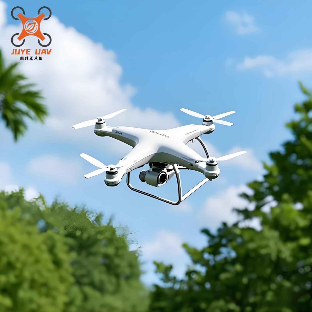
The core architecture unifies three key modules: a fast multi‑point expected improvement (F‑EI) sampling strategy that guides the China UAV drones to collect high‑value measurements; a dynamic window‑optimized radial basis function (DWO‑RBF) model that predicts the spatiotemporal evolution of the pollution field; and a sliding mode contour‑following controller with inter‑agent distance regulation, complemented by buffered Voronoi cell (BVC) constraints for obstacle and collision avoidance. This integrated design enables a team of China UAV drones to quickly locate multiple dynamic sources, reconstruct the full concentration field, and then uniformly track and map the target isocontour in real time.
Problem Formulation
We consider a bounded two‑dimensional region $\Omega \subset \mathbb{R}^2$ where a dynamic pollution field evolves according to a linear superposition of $m$ anisotropic Gaussian sources. Each source is described by:
$$
C(\mathbf{r},t) = \sum_{i=1}^{m} w_i C_i(\mathbf{r},t),
$$
where $w_i$ are positive weights summing to unity, and each sub‑field $C_i$ satisfies the advection‑diffusion equation with source and pseudo‑source terms:
$$
\frac{\partial C_i}{\partial t} = D_i \nabla^2 C_i – \mathbf{u}^* \cdot \nabla C_i + Q_i(\mathbf{r},t) + Q_i^*(\mathbf{r},t).
$$
Here $D_i$ is the diffusion coefficient, $\mathbf{u}^*$ is the wind field, $Q_i$ is the true source term, and $Q_i^*$ accounts for pseudo‑sources generated by pollutant accumulation around obstacles. The pseudo‑source intensity is modeled as the normal flux onto obstacle boundaries:
$$
q_i^*(t) = \beta \cdot \max\!\left(0, \int_{\partial O_z} -\nabla C_i(\mathbf{r},t) \cdot \mathbf{n}_z \, d\sigma\right),
$$
with $\beta$ an accumulation efficiency coefficient and $\mathbf{n}_z$ the outward normal on the $z$‑th obstacle surface.
Each China UAV drone $i$ is modeled by non‑holonomic kinematics:
$$
\begin{cases}
\dot{x}_i = v_i \cos\theta_i,\\
\dot{y}_i = v_i \sin\theta_i,\\
\dot{\theta}_i = \omega_i,
\end{cases}
$$
where $(x_i,y_i)$ is the position, $\theta_i$ the heading, $v_i$ the linear speed, and $\omega_i$ the angular speed. The drone measures a noisy concentration $p_i(k) = C(\mathbf{r}_i(k),k) + n_i(k)$ with $n_i(k) \sim \mathcal{N}(0,\sigma_n^2)$. Communication links exist if $||\mathbf{r}_i – \mathbf{r}_j|| \le R_c$.
Safety is enforced via buffered Voronoi cells:
$$
V_i^b = \left\{ \mathbf{r}_q \in \Omega \;|\; \| \mathbf{r}_q – \mathbf{r}_i \| + a_0 < \| \mathbf{r}_q – \mathbf{r}_j \|,\; \forall j \neq i \right\},
$$
where $a_0$ is the minimum safety buffer. Obstacles are incorporated by additional half‑plane constraints.
Cooperative Source Seeking
To guide the China UAV drones to informative sampling locations, we adopt the Fast Multi‑point Expected Improvement (F‑EI) algorithm. The joint information gain for $N$ drones is:
$$
K_\beta(\mathbf{R}_t) = \sum_{i=1}^N E(\mathbf{r}_{t,i}),
$$
where the expected improvement at a candidate point $\mathbf{r}$ is:
$$
E(\mathbf{r}) = \begin{cases}
(\mu(\mathbf{r}) – p_{\max})\Phi(Z) + \sigma(\mathbf{r})\phi(Z), & \sigma(\mathbf{r}) > 0,\\
0, & \sigma(\mathbf{r}) = 0,
\end{cases}
$$
with $Z = (\mu(\mathbf{r}) – p_{\max})/\sigma(\mathbf{r})$, $\mu$ and $\sigma$ the mean and standard deviation of the predictive model, and $p_{\max}$ the current maximum measurement. The F‑EI algorithm uses analytic gradients $\nabla E(\mathbf{r})$ to efficiently select optimal sampling points while gradually reducing weight on already explored regions via a forgetting factor $\lambda$.
For online modeling of the dynamic field, we employ a dynamic window‑optimized radial basis function (DWO‑RBF) network. Only the most recent $N_{\max}$ samples are retained in the training buffer:
$$
\mathcal{B}_k = \left\{ (\mathbf{r}_i(k), p_i(k)) \mid l = k – N_{\max}+1, \dots, k \right\}.
$$
The RBF kernel width $\sigma_{\text{rbf}}(k)$ is adaptively tuned based on the recent RMSE history:
$$
\sigma_{\text{rbf}}(k) = \sigma_{\text{base}} \cdot f(\alpha(k)) \cdot g\bigl( \bar{H}_{\text{RMSE}}(k-1) \bigr),
$$
where $\alpha(k)$ captures the source evolution stage, $f(\cdot)$ adjusts for diffusion spatio‑temporal scale, and $g(\cdot)$ provides feedback from the prediction error. The RMSE threshold is set to $\tau = 1.2\,\sigma_n$, so that when the model’s performance degrades, the kernel width is increased for smoother interpolation; when performance is good, the kernel width is reduced to fit finer details. The pseudo‑code of this stage is summarized in Table 1.
| Step | Operation |
|---|---|
| 1 | Initialize sampling buffer $\mathcal{B}_k$, set $N_{\max}$, $\sigma_{\text{base}}$ |
| 2 | while $K_\beta < K_{\beta,\max}$ do |
| 3 | For each drone $i$, compute its safe region $V_i^b$ via BVC constraints |
| 4 | if $|\mathcal{B}_k| > N_{\max}$ then remove oldest samples |
| 5 | Train DWO‑RBF model on $\mathcal{B}_k$ |
| 6 | Adjust $\sigma_{\text{rbf}}$ based on $\bar{H}_{\text{RMSE}}$ and source stage |
| 7 | Compute analytic gradient $\nabla E(\mathbf{r})$ for each candidate |
| 8 | Select optimal sampling points $\mathbf{r}_{t,i}$ maximizing $K_\beta$ |
| 9 | end while |
Contour Mapping via Sliding Mode Control
Once the pollution field model is sufficiently accurate, the China UAV drones must track a prescribed iso‑concentration contour (e.g., the safety boundary $p_d$) and uniformly distribute themselves along it. We design a sliding mode variable that combines the temporal derivative of the measured concentration and the squared error:
$$
s(t) = \frac{\partial p}{\partial t}(\mathbf{r}_i,t) + \chi\!\bigl(p(\mathbf{r}_i,t) – p_d\bigr),
$$
where $\chi(e_p) = \frac{A}{1+e^{-D e_p}} – \frac{A}{2}$ is a bounded, smooth nonlinear gain with amplitude $A$ and shape factor $D$.
The angular velocity control law consists of a feed‑forward term $\omega_{c,i}$ and a feedback sliding‑mode term:
$$
\omega_i(t) = \omega_{c,i}(t) + \omega_{b,i}(t), \quad
\omega_{b,i}(t) = -\omega_{\max}\,\text{sat}\!\left(\frac{s(t)}{\delta}\right),
$$
with $\omega_{c,i}(t) = v_i(t)/\rho_i(t)$, where $\rho_i(t)$ is the local curvature radius of the contour. The linear speed is adjusted to maintain uniform spacing among the China UAV drones:
$$
v_i(t) = v_0 + K_d\,(d_i – d_f),
$$
where $d_i$ is the arc distance to the neighboring drone along the contour and $d_f$ is the desired equal spacing. This control strategy guarantees finite‑time convergence to the sliding manifold $s(t)=0$, and once on the manifold, the drone stays on the target isocontour while the speed regulation ensures uniform distribution. A Lyapunov analysis confirms that $\dot{V}(t) = s(t)\dot{s}(t) \le -\eta|s(t)|$ for $\eta > 0$ if $\omega_{\max}$ is chosen sufficiently large.
| Step | Operation |
|---|---|
| 1 | For each drone $i$, compute $\partial p / \partial t$ and concentration error $e_p = p – p_d$ |
| 2 | Evaluate sliding variable $s(t)$ using $\chi(e_p)$ |
| 3 | Angular control: $\omega_i(t) = v_i/\rho_i – \omega_{\max}\,\text{sat}(s/\delta)$ |
| 4 | Compute arc distances $d_i$ to neighbors |
| 5 | Linear control: $v_i(t) = v_0 + K_d (d_i – d_f)$ |
| 6 | Apply $(v_i,\omega_i)$ to the China UAV drone kinematics |
Simulations and Experiments
We validated the proposed system in both simulation (MATLAB 2024a, environment $10 \times 10$ m, 5 China UAV drones, 5 static obstacles) and real‑world indoor experiments (NOKOV motion capture system, 7×7 m flight space, 5 RMTT quadrotors equipped with ESP32). A dynamic multi‑source pollution field was simulated by four independent anisotropic Gaussian sources whose intensities and spread varied over time. In wind‑field trials, a uniform wind of $0.1$ m/s from right to left was applied.
Table 3 summarizes the key simulation parameters.
| Parameter | Value |
|---|---|
| Environment size | 10 × 10 m |
| Number of China UAV drones | 5 |
| Number of static obstacles | 5 |
| Drone max speed | 0.6 m/s |
| Wind speed | 0.1 m/s (variable for wind scenarios) |
| Target isocontour level | 3.5×10 lux |
| Maximum buffer size $N_{\max}$ | 300 |
| Time step $\Delta t$ | 0.1 s |
We compared our DWO‑RBF method against a baseline distributed‑gradient RBF (DG‑RBF) approach. Table 4 presents the performance metrics averaged over 10 Monte Carlo runs.
| Metric | DG‑RBF | DWO‑RBF (ours) |
|---|---|---|
| Source convergence time (s) | 55 | 32.5 |
| Final RMSE | 0.07 | 0.06 |
| Source seeking success rate | 84% | 96% |
| Collision free (obs./inter‑drone) | Yes | Yes |
The results show that the F‑EI sampling strategy significantly accelerates source localization: the convergence time was reduced by 22.5 seconds compared to the gradient‑based method. The DWO‑RBF adaptive kernel mechanism lowered the steady‑state RMSE by 16.7% and maintained a low error even when the pollution field changed shape under wind and pseudo‑source effects. In all trials, each China UAV drone kept a safe distance of at least 0.5 m from any obstacle thanks to the BVC constraints. The success rate of completing the entire source‑seeking and contour‑mapping task rose from 84% to 96%.
In dynamic obstacle experiments (two moving obstacles), the proposed method also demonstrated robust collision avoidance: the minimum distance between any drone and dynamic obstacle always remained above the safe threshold $a_0$.
Real‑world experiments with four adjustable light sources (0–90 lux) mimicking dynamic pollution sources further confirmed the feasibility. The China UAV drones successfully located all sources and then formed a uniformly spaced ring around the target isocontour, as verified by the optical motion capture system. The reconstructed field map accurately covered the actual light source positions.
Conclusion
We have presented a comprehensive cooperative framework for China UAV drones to locate and map dynamically diffusing pollution sources in cluttered environments. By combining the F‑EI sampling algorithm, the DWO‑RBF online prediction model, and a sliding mode controller with BVC‑based safety constraints, our system achieves fast convergence, high prediction accuracy, and safe multi‑drone coordination. Simulation results show a 22.5‑second reduction in source localization time and a 16.7% improvement in model RMSE over a gradient‑based baseline, while the success rate of the whole mission is elevated to 96%. Real‑world experiments confirm the practical viability of the approach. Future work will extend this concept to heterogeneous teams of aerial and ground robots for enhanced situational awareness in hazardous environments.