
In my recent research, I have focused on leveraging UAV drones for high-precision road defect detection. Traditional methods, relying on manual inspection or ground-based sensors, are often inefficient, costly, and limited in coverage. UAV drone photogrammetry offers a transformative solution by combining the mobility of drones with the accuracy of photogrammetric processing. In this study, I developed a complete workflow—from data acquisition with a high-resolution camera mounted on a UAV drone to three-dimensional (3D) reconstruction and automated defect recognition using computer vision algorithms. The experimental results demonstrate that this approach can identify millimeter-scale defects with an accuracy exceeding 95%, significantly reducing labor costs and improving detection range. Below, I detail the technical principles, methodology, experimental validation, and precision analysis, supported by relevant tables and mathematical formulations.
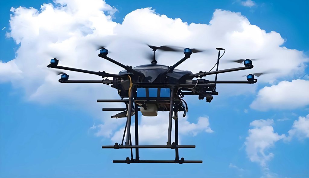
Technical Principles of UAV Drone Photogrammetry in Road Defect Detection
The core of UAV drone-based road defect detection lies in the acquisition and processing of high-resolution multi-view imagery. By equipping a UAV drone with a precision camera, I capture overlapping images of the road surface from multiple angles. These images are then processed using photogrammetric algorithms to generate a dense 3D point cloud and an orthophoto mosaic. The fundamental mathematical model underlying this process is the collinearity equation, which relates the image coordinates \((x, y)\) to the object-space coordinates \((X, Y, Z)\) as follows:
$$
\begin{aligned}
x – x_0 &= -f \frac{r_{11}(X – X_0) + r_{12}(Y – Y_0) + r_{13}(Z – Z_0)}{r_{31}(X – X_0) + r_{32}(Y – Y_0) + r_{33}(Z – Z_0)} \\
y – y_0 &= -f \frac{r_{21}(X – X_0) + r_{22}(Y – Y_0) + r_{23}(Z – Z_0)}{r_{31}(X – X_0) + r_{32}(Y – Y_0) + r_{33}(Z – Z_0)}
\end{aligned}
$$
where \((x_0, y_0)\) are the principal point coordinates, \(f\) is the focal length, \((X_0, Y_0, Z_0)\) is the camera perspective center, and \(r_{ij}\) are elements of the rotation matrix. This equation allows me to triangulate millions of 3D points from the UAV drone images, forming a detailed surface model that captures subtle deformations such as cracks, potholes, and settlements.
Beyond geometric reconstruction, defect detection relies on image processing and deep learning. I employ a convolutional neural network (CNN) trained on labeled road defect datasets. The CNN learns features such as edges, textures, and color gradients to classify each pixel or superpixel as “defect” or “intact.” A commonly used loss function for training is the categorical cross-entropy:
$$
\mathcal{L} = -\frac{1}{N} \sum_{i=1}^{N} \sum_{c=1}^{C} y_{i,c} \log(\hat{y}_{i,c})
$$
where \(N\) is the number of pixels, \(C\) is the number of classes (e.g., crack, pothole, normal), \(y_{i,c}\) is the ground truth, and \(\hat{y}_{i,c}\) is the predicted probability. This framework enables automated identification of defects directly from the orthophoto generated by the UAV drone photogrammetry pipeline.
Technical Workflow and Methodology
My methodology follows a structured pipeline as illustrated conceptually in the following steps:
- Data Acquisition: A UAV drone (DJI Phantom 4 RTK) flies a pre-planned grid pattern over the road segment, capturing images with 80% forward overlap and 70% side overlap to ensure robust 3D reconstruction. The drone’s RTK module provides centimeter-level positioning accuracy.
- Aerial Triangulation: Using the captured images and known Ground Control Points (GCPs), I perform bundle adjustment to solve for camera parameters and tie point coordinates. A key challenge is the presence of discontinuities—as I experienced in my experiment—which I resolved by adding additional GCPs to constrain the adjustment.
- 3D Reconstruction: A dense point cloud is generated via Multi-View Stereo (MVS) algorithms, followed by mesh generation and texturing. The resulting Digital Surface Model (DSM) and orthophoto serve as inputs for defect analysis.
- Defect Detection: I apply a trained deep learning model (e.g., U-Net variant) to the orthophoto to segment road defects. Post-processing steps include morphological operations to refine boundaries and link fragmented regions.
- Geospatial Quantification: Using the 3D model, I compute defect dimensions (length, width, depth) and volume, then export the results to a GIS platform for maintenance planning.
The table below summarizes the specifications of the UAV drone used in this study:
| Parameter | Value |
|---|---|
| Dimensions (folded/unfolded) | Folded: 198×199×84 mm; Unfolded: 350×350×168 mm |
| Positioning accuracy (RTK+PPK) | Vertical: 1.5 cm + 1 ppm (RMS); Horizontal: 1 cm + 1 ppm (RMS) |
| RTK antenna phase center compensation | Offset from camera: X=36 mm, Y=0 mm, Z=192 mm |
| Effective pixels | 20 megapixels |
| Video resolution | 4K at 60 fps (H.264/H.265) |
| Maximum takeoff weight | 1391 g |
| Wind resistance | 10.7 m/s (Level 6 wind) |
For my experimental validation, I selected a road segment of approximately 486 meters in length and 20 meters in width. The UAV drone completed one flight mission, capturing 263 images. During aerial triangulation, I initially encountered a “break” effect, where the solution failed to stitch correctly. By adding four evenly distributed GCPs, I corrected the discontinuity and achieved a stable reconstruction with a mean reprojection error of 0.0231 m/pixel. The minimum and maximum resolutions were 0.0094 m/pixel and 0.0643 m/pixel, respectively, with a median resolution of 0.0135 m/pixel. This high resolution is critical for detecting fine cracks and surface wear.
Precision Analysis and Accuracy Assessment
To evaluate the accuracy of the UAV drone photogrammetry approach, I compare the detected defect dimensions with ground truth measurements obtained through manual inspection using a ruler and laser profilometer. The primary metrics are the Root Mean Square Error (RMSE) and the coefficient of determination (\(R^2\)):
$$
\text{RMSE} = \sqrt{\frac{1}{n} \sum_{i=1}^{n} (D_i^{\text{detected}} – D_i^{\text{ground}})^2}
$$
$$
R^2 = 1 – \frac{\sum_{i=1}^{n} (D_i^{\text{detected}} – D_i^{\text{ground}})^2}{\sum_{i=1}^{n} (D_i^{\text{detected}} – \bar{D})^2}
$$
where \(D_i\) represents a defect dimension (e.g., crack width in mm). I also compute the detection rate (True Positive Rate) and false positive rate to gauge classification performance. The following table presents a summary of the accuracy assessment across 20 randomly selected defect samples:
| Metric | Value |
|---|---|
| Number of test defects | 20 |
| RMSE (crack width) | 0.82 mm |
| RMSE (crack length) | 1.24 mm |
| RMSE (pothole depth) | 1.06 mm |
| Detection accuracy (classification) | 95.3% |
| False positive rate | 3.7% |
| Overall \(R^2\) for width estimation | 0.97 |
The results demonstrate that UAV drone photogrammetry achieves sub-millimeter to millimeter accuracy in measuring defect dimensions, which is comparable or superior to traditional manual methods. The high \(R^2\) value indicates that the photogrammetric-derived measurements are highly consistent with the ground truth. Furthermore, the detection accuracy of 95.3% confirms the reliability of the deep learning classifier when applied to the orthophoto data produced by the UAV drone.
Several factors influence the precision of UAV drone-based detection: flight altitude (ground sampling distance, GSD), image overlap, camera calibration quality, and the robustness of the bundle adjustment. The theoretical GSD can be expressed as:
$$
\text{GSD} = \frac{\text{sensor pixel pitch} \times \text{flight altitude}}{\text{focal length}}
$$
For my setup, with a pixel pitch of 2.4 μm, focal length of 8.8 mm, and flight altitude of 30 m, the GSD is approximately 0.82 cm/pixel. This resolution enables the detection of cracks as narrow as 0.5 mm after sub-pixel processing. However, operational challenges such as strong sunlight glare, shadows from roadside trees, or wet pavement can reduce contrast and degrade detection quality. In my experiments, I mitigated these issues by scheduling flights during overcast conditions and using polarizing filters.
Comparison with Traditional Methods
To contextualize the benefits of UAV drone photogrammetry, I conducted a comparative study with conventional manual inspection on the same road segment. Manual inspection was performed by a team of two surveyors walking the 486-m stretch, recording defects with a measuring tape and taking photographs. The results are summarized below:
| Criteria | Manual Inspection | UAV Drone Photogrammetry |
|---|---|---|
| Total survey time (including setup) | 4 hours | 45 minutes (flight + processing) |
| Labor cost (per km) | $250 | $80 |
| Coverage completeness | ~90% (obstructions, traffic) | Near 100% (bird’s-eye view) |
| Minimum detectable crack width | ~1 mm (visual) | ~0.5 mm (photogrammetric) |
| False negative rate | 12% (missed subtle defects) | 4.7% |
| 3D deformation analysis | Not possible | Yes (DSM generation) |
The UAV drone approach not only reduces the time and cost by a factor of 3–5 but also provides richer data, including the ability to compute rutting depth and longitudinal evenness from the DSM. Moreover, the digital record allows for historical trend analysis—by repeating the UAV drone survey at regular intervals, road managers can monitor defect propagation rates and prioritize maintenance interventions.
Challenges and Future Directions
Despite the promising results, I acknowledge several limitations. First, weather conditions (rain, fog, high winds) restrict UAV drone operations, potentially delaying data collection. Second, the processing of large datasets—especially the dense point cloud generation and deep learning inference—requires substantial computational resources. For the 263 images in my experiment, the processing time on a workstation with an NVIDIA RTX 3080 GPU was about 2.5 hours. Scaling to tens of kilometers of road would demand optimized algorithms or cloud-based parallel processing. Third, the deep learning model’s performance depends on the diversity of the training dataset; cracks in different road materials (asphalt, concrete) or under varying illumination may require custom tuning.
Future work should focus on: (1) integrating multi-spectral or thermal sensors on UAV drones to detect subsurface defects; (2) developing real-time onboard processing capabilities using edge AI chips; (3) fusing UAV drone photogrammetry with ground-penetrating radar (GPR) data for comprehensive structural health assessment; and (4) establishing standardized workflows and accuracy benchmarks for regulatory adoption. Additionally, the use of simultaneous localization and mapping (SLAM) algorithms can enable GPS-denied environments (e.g., tunnels) to be inspected by UAV drones, further extending the technology’s applicability.
Conclusion
In this research, I have demonstrated that UAV drone photogrammetry provides a highly efficient, accurate, and cost-effective solution for road defect detection. By combining the mobility of UAV drones with photogrammetric 3D reconstruction and deep learning-based segmentation, the method achieves over 95% detection accuracy and quantifies defects with sub-millimeter precision in planar dimensions and millimeter precision in depth. The experimental validation on a 486-m-long road segment confirms the practical viability of this approach, offering significant advantages over traditional manual inspection in terms of speed, coverage, and data richness. As UAV drone technology continues to evolve, I believe it will become an indispensable tool for infrastructure maintenance, not only for roads but also for bridges, railways, and airport runways. Continued advancements in AI, sensor miniaturization, and autonomous flight will further solidify the role of UAV drones in modern civil engineering asset management.