
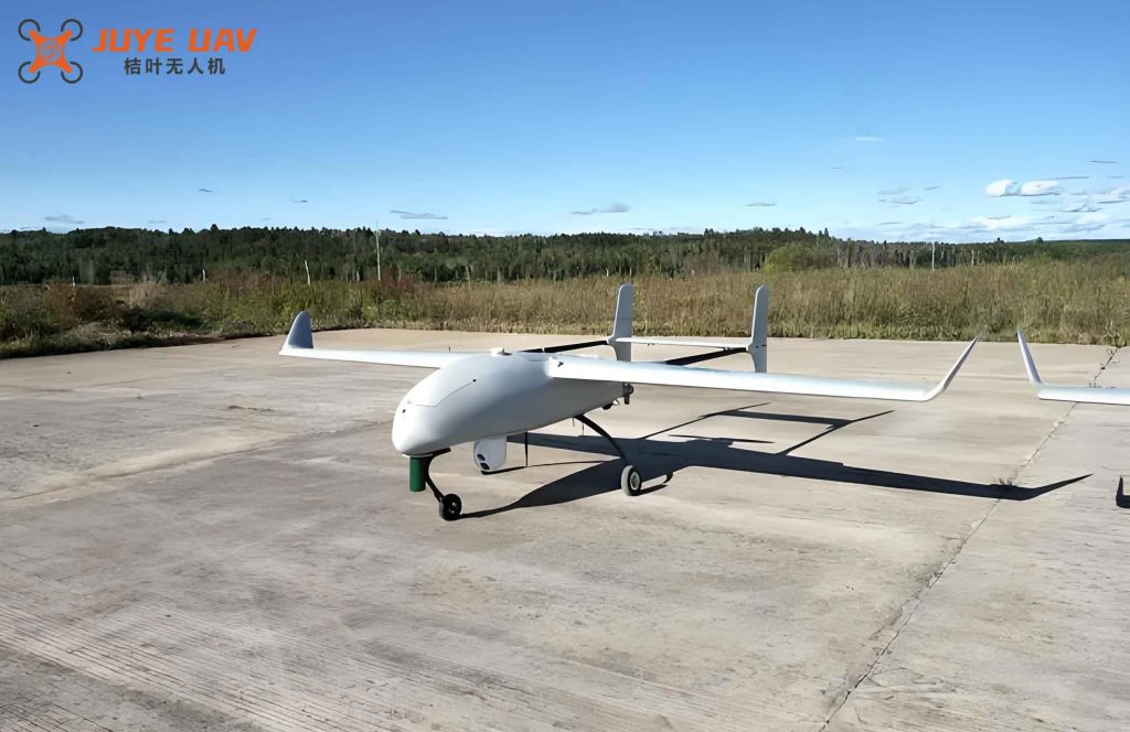
In the context of modern warfare evolving towards informatization, unmanned and intelligent systems, military fixed-wing UAVs are rapidly proliferating worldwide and becoming a key procurement direction for future weaponry. Meanwhile, the industrial-grade fixed-wing UAV market is growing quickly due to technological maturity and government policy support. Civil applications such as agricultural plant protection, power line inspection, aerial surveying, and police security are continuously expanding. Advances in fixed-wing UAV technology drive higher-altitude operations, longer-range control, higher flight speeds, and extended endurance. Compared to other UAV types, fixed-wing UAVs offer high maneuverability, long endurance, and broader application scenarios.
Classic PID control is widely used in flight control due to its simplicity, robustness, and ease of tuning. However, environmental disturbances, system parameter variations, and measurement noise degrade PID performance for fixed-wing UAVs. Therefore, integrating modern control theory with traditional methods is a trend. Various advanced approaches have been applied to optimize PID controllers and handle system uncertainties. For example, fuzzy logic parameter self-tuning enhances dynamic response and anti-interference capability compared to classic PID. Genetic algorithms optimize PID parameters through iterative search, reducing control time and improving accuracy. Reinforcement learning with neural networks simulates PID behavior, exploring optimal strategies under given conditions. Sliding mode control addresses modeling difficulties by being insensitive to uncertainties and disturbances. Adaptive control fusion is also a hot research area, with adaptive update strategies handling input delays and real-time estimation of uncertain parameters. Recursive least squares algorithms provide precise parameter identification and uncertainty estimation. Adaptive update rate mechanisms adjust uncertain parameters in real time for constrained systems.
To ensure precise and stable flight trajectory tracking for fixed-wing UAVs, we design an adaptive model predictive control (MPC) law. This makes the MPC algorithm more general, adaptable to various operating environments, diverse control requirements, and different tracking paths. By continuously updating the system model, the controller outputs optimal control inputs to the actuators, achieving more accurate control. We focus on tracking the descent phase trajectory for altitude control.
1. Longitudinal Channel Mathematical Model
The controlled plant is a 700 kg class fixed-wing UAV. Considering the complexity of motion and coupling between aerodynamic and control channels, we adopt reasonable assumptions: the airframe is rigid, symmetrical, and mass distribution is uniform. Based on rigid body kinematics and coordinate transformations, we obtain a six-degree-of-freedom nonlinear dynamic and kinematic model. Using small perturbation theory, we decouple longitudinal and lateral movements and linearize. The resulting longitudinal linear continuous state-space model is:
$$
\begin{aligned}
\dot{x} &= A x + B u \\
y &= C x + D u
\end{aligned}
$$
where
$$
A = \begin{bmatrix}
a_{11} & a_{12} & a_{13} & a_{14} & a_{15} \\
a_{21} & a_{22} & a_{23} & a_{24} & a_{25} \\
a_{31} & a_{32} & a_{33} & a_{34} & a_{35} \\
a_{41} & a_{42} & a_{43} & a_{44} & a_{45} \\
a_{51} & a_{52} & a_{53} & a_{54} & a_{55}
\end{bmatrix}, \quad
B = \begin{bmatrix}
b_{11} \\
b_{21} \\
b_{31} \\
b_{41} \\
b_{51}
\end{bmatrix}, \quad
C = \begin{bmatrix}
1 & 0 & 0 & 0 & 0 \\
0 & 1 & 0 & 0 & 0 \\
0 & 0 & 1 & 0 & 0 \\
0 & 0 & 0 & 1 & 0 \\
0 & 0 & 0 & 0 & 1
\end{bmatrix}, \quad
D = \begin{bmatrix}
0 \\
0 \\
0 \\
0 \\
0
\end{bmatrix}
$$
Here, the input \( u = \delta_e \) (elevator deflection), and the state vector \( x = [\Delta V,\ \Delta h,\ \Delta q,\ \Delta \theta,\ \Delta \alpha]^T \) represents changes in velocity, altitude, pitch rate, pitch angle, and angle of attack, respectively. The system is a single-input multiple-output (SIMO) system. During simulation, we superimpose a constant airspeed of 35 m/s on the velocity output.
2. Adaptive MPC Control
2.1 Model Predictive Control (MPC) Logic
The adaptive MPC architecture consists of three parts: an MPC controller, a fixed-wing UAV longitudinal model, and an adaptive parameter update mechanism. The MPC controller is the core for flight trajectory tracking. It solves a finite-horizon optimal control problem based on a predefined altitude reference trajectory and a cost function, generating optimal control inputs to the UAV’s longitudinal dynamics. The initial state is fed into the MPC controller to predict future states, and this process repeats for tracking.
2.2 MPC Controller Design
2.2.1 Linear Error Model
We describe the fixed-wing UAV model in state-space form. Discretizing at time step \( k \) gives:
$$
\begin{aligned}
x(k+1) &= A_d x(k) + B_d u(k) \\
y(k) &= C_d x(k) + D_d u(k)
\end{aligned}
$$
where \( x(k) \in \mathbb{R}^5 \), \( A_d \in \mathbb{R}^{5 \times 5} \), \( B_d \in \mathbb{R}^{5 \times 1} \), \( C_d \in \mathbb{R}^{5 \times 5} \), \( D_d = 0 \). To formulate an incremental model, we define:
$$
\begin{aligned}
\Delta x(k) &= x(k) – x(k-1) \\
\Delta u(k) &= u(k) – u(k-1) \\
y(k) &= C_d x(k)
\end{aligned}
$$
Then the incremental system is:
$$
\begin{aligned}
\Delta x(k+1) &= A_d \Delta x(k) + B_d \Delta u(k) \\
y(k) &= y(k-1) + C_d \Delta x(k)
\end{aligned}
$$
Introduce prediction horizon \( p \) and control horizon \( m \). Assume:
$$
\begin{aligned}
\Delta u(k+i) &= 0, \quad i = m, m+1, \dots, p-1 \\
\end{aligned}
$$
Then the predicted state increments are:
$$
\begin{aligned}
\Delta x(k+1|k) &= A_d \Delta x(k) + B_d \Delta u(k) \\
\Delta x(k+2|k) &= A_d^2 \Delta x(k) + A_d B_d \Delta u(k) + B_d \Delta u(k+1) \\
&\vdots \\
\Delta x(k+p|k) &= A_d^p \Delta x(k) + \sum_{i=0}^{p-1} A_d^{p-1-i} B_d \Delta u(k+i)
\end{aligned}
$$
Define vectors:
$$
\begin{aligned}
X &= [\Delta x(k+1|k)^T, \Delta x(k+2|k)^T, \dots, \Delta x(k+p|k)^T]^T \\
\Delta U &= [\Delta u(k)^T, \Delta u(k+1)^T, \dots, \Delta u(k+m-1)^T]^T
\end{aligned}
$$
Then:
$$
X = F \Delta x(k) + G \Delta U
$$
where
$$
F = \begin{bmatrix}
A_d \\
A_d^2 \\
\vdots \\
A_d^p
\end{bmatrix},\quad
G = \begin{bmatrix}
B_d & 0 & \cdots & 0 \\
A_d B_d & B_d & \cdots & 0 \\
\vdots & \vdots & \ddots & \vdots \\
A_d^{p-1} B_d & A_d^{p-2} B_d & \cdots & \sum_{j=0}^{p-m} A_d^j B_d
\end{bmatrix}
$$
Similarly, the predicted outputs are:
$$
Y = \begin{bmatrix}
y(k+1|k) \\
y(k+2|k) \\
\vdots \\
y(k+p|k)
\end{bmatrix} = \Phi y(k) + \Psi \Delta x(k) + \Theta \Delta U
$$
with appropriate matrices \( \Phi, \Psi, \Theta \). The output prediction can be expressed in terms of current measured output \( y(k) \), current state increment \( \Delta x(k) \), and future control increments \( \Delta U \).
2.2.2 Cost Function Design
The optimization considers: (1) tracking the reference input, and (2) minimizing control effort. Since we aim to drive the output \( y \) to zero reference (setpoint tracking can be reformulated), define error \( E(k) = -y(k) \) (assuming reference is zero). The cost function is:
$$
J = \sum_{i=1}^{p} E(k+i|k)^T Q E(k+i|k) + \sum_{i=0}^{m-1} \Delta u(k+i)^T R \Delta u(k+i) + E(k+p|k)^T P E(k+p|k)
$$
where \( Q \) and \( R \) are diagonal weighting matrices, and \( P \) is the terminal weight. In the unconstrained case, we can convert to:
$$
J = \frac{1}{2} \Delta U^T H \Delta U + \Delta U^T f
$$
with
$$
H = 2 ( \Theta^T \bar{Q} \Theta + \bar{R} ), \quad f = 2 ( \Theta^T \bar{Q} ( \Phi y(k) + \Psi \Delta x(k) ) )
$$
Here \( \bar{Q} = \text{diag}(Q, \dots, Q, P) \), \( \bar{R} = \text{diag}(R, \dots, R) \). The optimal solution is:
$$
\Delta U^* = -H^{-1} f
$$
Only the first element \( \Delta u(k) \) is applied.
2.2.3 Constraints
We constrain elevator deflection and its rate to maintain flight stability:
$$
\begin{aligned}
-10^\circ &\leq \delta_e \leq 10^\circ \\
-5 \text{ rad/s} &\leq \dot{\delta}_e \leq 5 \text{ rad/s}
\end{aligned}
$$
In discrete form:
$$
\begin{aligned}
u_{\min} &\leq u(k+i) \leq u_{\max}, \quad i=0,\dots,m-1 \\
\Delta u_{\min} &\leq \Delta u(k+i) \leq \Delta u_{\max}, \quad i=0,\dots,m-1
\end{aligned}
$$
The prediction horizon \( p \) significantly affects performance. We simulate different horizons and observe the results. A summary of the effect is shown in Table 1.
| Prediction Horizon \( p \) | Response Speed | Overshoot | Oscillation |
|---|---|---|---|
| 5 | Fast | Large | Yes |
| 8 | Fast | None | None |
| 10 | Moderate | None | None |
| 15 | Slow | None | None |
Similarly, varying control horizon \( m \) with fixed \( p=8 \) yields:
| Control Horizon \( m \) | Response Speed | Overshoot/Oscillation |
|---|---|---|
| 1 | Fast | Significant overshoot |
| 2 | Fast | None |
| 3 | Fast | Some overshoot |
| 4 | Moderate | Lag and overshoot |
Based on these simulations, we select the MPC parameters as shown in Table 3.
| Parameter | Value |
|---|---|
| Prediction horizon \( p \) | 8 |
| Control horizon \( m \) | 2 |
| Sampling period \( T_s \) | 0.15 s |
| Elevator deflection limits | [-20°, 20°] (≈ ±0.349 rad) |
| Elevator deflection rate limits | [-5 rad/s, 5 rad/s] |
| Weight on output error \( Q \) | \( \text{diag}(800, 1, 1, 1, 1) \) (altitude weight large) |
| Weight on control increment \( R \) | 10 |
| Reference sequence | [180, 0, 0, 0, 0]^T (altitude reference 180 m) |
2.3 Adaptive Update Rate Design
2.3.1 Estimator Design
Consider the discrete system in (2). We design an estimator for the state:
$$
\hat{x}(k+1) = \hat{A}(k) \hat{x}(k) + \hat{B}(k) u(k)
$$
where \( \hat{A} \) and \( \hat{B} \) are estimates of system matrices. Define state estimation error \( \tilde{x}(k) = x(k) – \hat{x}(k) \). Then:
$$
\tilde{x}(k+1) = A x(k) + B u(k) – \hat{A}(k) \hat{x}(k) – \hat{B}(k) u(k)
$$
Introduce parameter estimation error \( \tilde{a}(k) = a – \hat{a}(k) \), where \( a = [A, B] \) and \( \hat{a} = [\hat{A}, \hat{B}] \). Define regressor \( \Theta(k) = [x(k)^T, u(k)^T]^T \). Then:
$$
\tilde{x}(k+1) = \tilde{a}(k) \Theta(k)
$$
Note that \( \tilde{a}(k) \in \mathbb{R}^{5 \times 6} \).
2.3.2 Adaptive Update Law
To keep parameter estimation errors bounded and drive state estimation errors to zero, we design a gradient-based adaptive update law. The cost function at time \( k \) is:
$$
J_a(k) = \tilde{x}(k+1)^T \tilde{x}(k+1)
$$
The gradient with respect to \( \hat{a}(k) \) is:
$$
\nabla_{\hat{a}} J_a(k) = -2 \tilde{x}(k+1) \Theta(k)^T
$$
We update the parameter estimate using:
$$
\hat{a}(k+1) = \hat{a}(k) – \lambda(k) \nabla_{\hat{a}} J_a(k)
$$
To choose the step size \( \lambda(k) \), we minimize \( J_a(k+1) \) with respect to \( \lambda(k) \) yielding:
$$
\lambda(k) = \frac{1}{2 \|\Theta(k)\|^2}
$$
Thus the adaptive update law is:
$$
\hat{a}(k+1) = \hat{a}(k) + \frac{1}{\|\Theta(k)\|^2} \tilde{x}(k+1) \Theta(k)^T
$$
This adaptive mechanism updates the model used by the MPC controller in real time, improving tracking accuracy even under changing conditions.
3. Simulation and Analysis
We implemented the adaptive MPC controller in Simulink for the fixed-wing UAV longitudinal dynamics. The simulation model includes the MPC controller, the UAV model, and the adaptive parameter update block. The desired altitude trajectory for landing is shown in Figure 1 (conceptual: descent from 160 m to 60 m, level flight at 60 m, then flare to ground). We use the MPC parameters from Table 3.
The simulation results are presented below. The adaptive MPC tracking performance is compared to a classic PID controller.
| Controller | Max Absolute Error (m) | RMS Error (m) |
|---|---|---|
| Classic PID | 0.52 | 0.18 |
| Adaptive MPC | 0.40 | 0.12 |
The adaptive MPC reduces the maximum tracking error by about 23% compared to PID. The error remains bounded and does not diverge, demonstrating good convergence and robustness.
The control input (elevator deflection) remains within the prescribed limits. The adaptive MPC yields smoother control actions, avoiding aggressive oscillations seen in PID under certain conditions.
4. Conclusion
We have presented an adaptive model predictive control design for longitudinal altitude tracking of a fixed-wing UAV. The approach integrates a linear state-space model, receding horizon optimization with constraints, and an online adaptive update law that adjusts the system matrices based on estimation errors. Simulation results confirm that the adaptive MPC provides superior tracking accuracy compared to classic PID, with a 23% reduction in maximum altitude error. The controller maintains stability and responds quickly to reference changes without overshoot.
The adaptive MPC leverages real-time model updates to handle uncertainties and environmental variations, making it suitable for fixed-wing UAV operations in diverse scenarios. Future work will introduce external disturbances and test the controller in more realistic flight conditions, including wind gusts and sensor noise.