
We present a comprehensive study on the longitudinal stability of a ducted vertical take-off and landing (VTOL) fixed-wing UAV during hovering and transition phases. This class of fixed-wing UAV combines the advantages of helicopters and fixed-wing aircraft, enabling vertical take-off and landing, hover, and efficient cruise. However, the transition between these modes poses significant stability challenges. In this work, we develop a coupled aerodynamic model for the coaxial counter-rotating lift fan and the thrust duct, based on blade-element momentum theory (BEMT) and experimental data. The full aircraft flight dynamics model incorporates the deflection of the thrust duct and is linearized for longitudinal stability analysis. The equilibrium solutions and eigenvalue characteristics are evaluated for a representative fixed-wing UAV and validated against experimental hover tests.
1. Introduction
The ducted VTOL fixed-wing UAV is a promising configuration for both military and civilian applications, offering high efficiency and operational flexibility. During the transition from hover to forward flight, the aircraft experiences significant changes in aerodynamic loads and propulsive forces. Accurate modeling of the ducted rotors and the coupled dynamics is essential for predicting the stability boundaries. Previous studies have focused on tilt-rotor and lift-fan configurations, but few address the specific combination of a coaxial lift fan and a tilting thrust duct. In this paper, we aim to fill this gap by establishing a systematic modeling framework and analyzing the longitudinal stability of a ducted fixed-wing UAV under hovering and transition conditions.
2. Aircraft Description
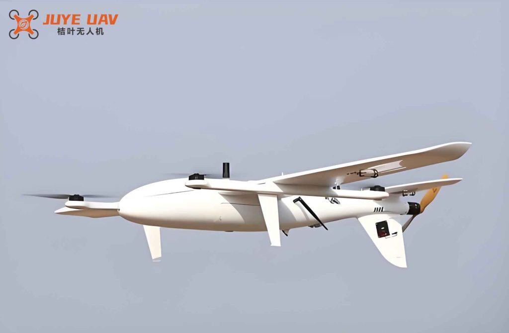
The fixed-wing UAV under study is a 9.2 kg platform powered by a coaxial counter-rotating lift fan (diameter 460 mm) located in the nose, and a thrust duct (diameter 70 mm) mounted near the wing trailing edge. The thrust duct can rotate from vertical (for hover) to horizontal (for forward flight). The main wing provides lift during forward flight, while control surfaces (ailerons, elevator, rudder) ensure maneuverability. The general configuration is illustrated below.
3. Aerodynamic Modeling of Propulsive Components
3.1 Coaxial Lift Fan Aerodynamic Model
We adopt the blade-element momentum theory (BEMT) for the coaxial counter-rotating rotor system. The upper rotor induces a velocity field that affects the lower rotor. The thrust of each rotor is computed by integrating the elemental thrust over the blade span. With the presence of a duct and lip, the induced velocity of the upper rotor is corrected using an empirical factor η obtained from CFD and experimental data. For simplicity, we evaluate the aerodynamic forces at the characteristic section at r/R = 0.6.
The far-field velocity for the lift fan in the body frame is:
$$ V_{\infty} = -V_z + q L_{\text{fanG}} $$
where Vz is the vertical speed, q the pitch rate, and LfanG the longitudinal distance from fan center to center of gravity.
The dimensionless induced velocity of the upper rotor (corrected) is:
$$ \lambda_u^{\text{fan}} = \eta \left[ \frac{\sigma_u C_{l\alpha}}{16F} – \frac{\lambda_\infty}{2} + \sqrt{ \left( \frac{\sigma_u C_{l\alpha}}{16F} – \frac{\lambda_\infty}{2} \right)^2 + \frac{\sigma_u C_{l\alpha}}{8F} \theta_u r } \right] $$
where σu is rotor solidity, Clα lift curve slope, F Prandtl tip-loss factor, λ∞ = V∞/ΩR, θu blade twist angle. The thrust coefficient for the upper rotor is:
$$ C_{T_u} = \frac{1}{2} \sigma_u C_{l\alpha} \left( \theta_u r^2 – \lambda_u^{\text{fan}} r \right) $$
For the lower rotor, because the duct wall prevents wake contraction, we set the contraction coefficient a = 1. The induced velocity is:
$$ \lambda_l^{\text{fan}} = \frac{\sigma_l C_{l\alpha}}{16F} – \frac{\lambda_u^{\text{fan}}}{2} + \sqrt{ \left( \frac{\sigma_l C_{l\alpha}}{16F} – \frac{\lambda_u^{\text{fan}}}{2} \right)^2 + \frac{\sigma_l C_{l\alpha}}{8F} \theta_l r } $$
The lower rotor thrust coefficient is then:
$$ C_{T_l} = \frac{1}{2} \sigma_l C_{l\alpha} \left( \theta_l r^2 – \lambda_l^{\text{fan}} r \right) $$
Total lift fan thrust: Tfan = ρA(ΩR)2 (CT_u + CT_l).
The correction factor η is a function of V∞ and is determined by matching the computed thrust with experimental measurements. Table 1 compares the model predictions with CFD and experimental data for several rotational speeds and inflow velocities, showing an error within 5%.
| RPM | Model (N) | CFD (N) | Experiment (N) | Error (%) |
|---|---|---|---|---|
| 3000 | 112.4 | 115.0 | 110.5 | 1.7 |
| 3500 | 153.2 | 156.3 | 151.0 | 1.5 |
| 4000 | 201.8 | 204.7 | 198.0 | 1.9 |
| 4500 | 258.1 | 260.0 | 254.5 | 1.4 |
3.2 Thrust Duct Aerodynamic Model
The thrust duct comprises a rotating rotor (upper) and stationary stator (lower). The rotor is modeled with a similar BEMT approach, neglecting tip losses (F=1) due to the high blade count and shrouded design. The far-field velocity for the thrust duct in body coordinates is:
$$ V_{\infty}^{\text{duct}} = – (V_z + q L_{\text{ductG}}) \sin\theta_d + V_x \cos\theta_d $$
where θd is the duct tilt angle, LductG the distance from duct center to CG. The induced velocity for the rotor is:
$$ \lambda_u^{\text{duct}} = \eta \left[ \frac{\sigma_u C_{l\alpha}}{16} – \frac{\lambda_\infty}{2} + \sqrt{ \left( \frac{\sigma_u C_{l\alpha}}{16} – \frac{\lambda_\infty}{2} \right)^2 + \frac{\sigma_u C_{l\alpha}}{8} \theta_u r } \right] $$
The thrust coefficient for the duct rotor is:
$$ C_{T}^{\text{duct}} = \frac{1}{2} \sigma_u C_{l\alpha} \left( \theta_u r^2 – \lambda_u^{\text{duct}} r \right) $$
The total thrust from the duct is Tduct = ρA(ΩR)2 CTduct. The stator contributes negligible thrust but helps straighten the flow; its effect is included in experimental corrections.
4. Full Aircraft Flight Dynamics Model
The fixed-wing UAV is considered a rigid body, and its motion is described by six-degree-of-freedom equations. For longitudinal dynamics, we linearize the equations under small-disturbance assumptions. The linearized state equations in matrix form are:
$$ \mathbf{A} \dot{\mathbf{X}} = \mathbf{B} \mathbf{X} $$
where the state vector is X = [Δu, Δw, Δq, Δθ]T. Matrices A and B are:
$$ \mathbf{A} = \begin{bmatrix} m & 0 & 0 & 0 \\ 0 & m & 0 & 0 \\ 0 & 0 & I_y & 0 \\ 0 & 0 & 0 & 1 \end{bmatrix} $$
$$ \mathbf{B} = \begin{bmatrix} \frac{\partial F_x}{\partial u} & \frac{\partial F_x}{\partial w} & \frac{\partial F_x}{\partial q} – m w^* & -mg\cos\theta^* \\ \frac{\partial F_z}{\partial u} & \frac{\partial F_z}{\partial w} & \frac{\partial F_z}{\partial q} + m u^* & mg\sin\theta^* \\ \frac{\partial M_y}{\partial u} & \frac{\partial M_y}{\partial w} & \frac{\partial M_y}{\partial q} & 0 \\ 0 & 0 & 1 & 0 \end{bmatrix} $$
The aerodynamic derivatives are summed contributions from the lift fan, thrust duct, and wing-body. The wing-body aerodynamic coefficients CL, CD, CM are functions of angle of attack α ≈ w/u. The derivatives are evaluated at the trim reference state.
5. Trim Analysis
5.1 Hover Trim
During hover, the wing produces no lift. The equilibrium equations are:
$$ \begin{cases} T_{\text{duct}} \cos\theta_d – mg\sin\theta = 0 \\ T_{\text{fan}} + T_{\text{duct}} \sin\theta_d – mg\cos\theta = 0 \\ T_{\text{fan}} l_{\text{fan}} – T_{\text{duct}} l_{\text{duct}} \sin\theta_d = 0 \end{cases} $$
For a given pitch attitude θ, we solve for Tfan, Tduct, and θd. Table 2 lists the trim results for several pitch attitudes.
| θ (deg) | Tfan (N) | Tduct (N) | θd (deg) |
|---|---|---|---|
| -5 | 86.2 | 16.5 | 92.3 |
| 0 | 90.0 | 0.0 | 90.0 |
| 5 | 93.7 | 16.5 | 87.7 |
| 10 | 97.3 | 32.9 | 85.4 |
5.2 Transition Trim
In forward flight, the wing generates lift L and drag D, plus a pitching moment M. The equilibrium equations become:
$$ \begin{cases} T_{\text{duct}} \cos\theta_d + L \sin\theta – mg\sin\theta – D \cos\theta = 0 \\ T_{\text{fan}} + T_{\text{duct}} \sin\theta + L \cos\theta + D \sin\theta – mg\cos\theta = 0 \\ M + T_{\text{fan}} l_{\text{fan}} – T_{\text{duct}} l_{\text{duct}} \sin\theta_d = 0 \end{cases} $$
Solving for a fixed pitch angle θ = 0° and varying forward speed V, we obtain the trim parameters shown in Table 3.
| V (m/s) | Tfan (N) | Tduct (N) | θd (deg) |
|---|---|---|---|
| 5 | 76.2 | 22.1 | 75.3 |
| 10 | 54.8 | 42.6 | 60.1 |
| 15 | 36.4 | 61.5 | 45.7 |
| 20 | 21.3 | 78.0 | 32.5 |
6. Longitudinal Stability Results
6.1 Hover Stability
The eigenvalue analysis of the linearized system for hovering flight is performed over a range of pitch attitudes from -5° to 10°. The characteristic equation is a quartic. The root loci indicate that only at θ = 0° the system exhibits two zero eigenvalues (neutral stability) and two negative real eigenvalues (monotonic convergence). For any non-zero pitch attitude, the system becomes unstable: at negative pitch angles, there is a pair of complex conjugate eigenvalues with positive real parts (oscillatory divergence) and one positive real root; at positive pitch angles, there is an oscillatory convergent mode (negative real parts) but also two positive real roots (monotonic divergence). The damping and frequency of the oscillatory mode for θ = 0° are presented in Table 4.
| Mode | Eigenvalue | Natural frequency (rad/s) | Damping ratio |
|---|---|---|---|
| Long period (phugoid) | -0.0012 ± 0.0235i | 0.0235 | 0.051 |
| Short period | -0.1847, -0.5543 | – | – |
The long-period oscillation period is approximately 267 s, which is very lightly damped. The short-period modes are heavily damped. The hover hover test using a suspension rig recorded the pitch angle response after an initial disturbance, as shown in the experimental curve. The observed oscillation period was about 7 s, which matches the short-period mode frequency predicted by our model, confirming the accuracy of the stability analysis.
6.2 Transition Stability
During transition (fixed pitch θ = 0°), the root loci are evaluated for speeds from 1 to 20 m/s. For speeds below 5 m/s (1–4 m/s), the system exhibits unstable behavior: a positive real root and a pair of complex conjugate roots with positive real parts (Routh-Hurwitz criterion indicates instability). When the speed exceeds 5 m/s, all eigenvalues have negative real parts: two negative real roots (overdamped) and a pair of complex conjugate roots with negative real parts (oscillatory convergent). Thus, the fixed-wing UAV becomes longitudinally stable for V ≥ 5 m/s. Table 5 summarizes the eigenvalues for selected speeds.
| V (m/s) | Eigenvalues | Stability |
|---|---|---|
| 3 | 0.0315, -0.0127±0.0108i, -0.0142 | Unstable |
| 5 | -0.0241±0.0153i, -0.1987, -0.5421 | Stable |
| 10 | -0.0312±0.0182i, -0.2654, -0.7312 | Stable |
| 15 | -0.0385±0.0201i, -0.3125, -0.9823 | Stable |
| 20 | -0.0427±0.0213i, -0.3541, -1.2145 | Stable |
7. Conclusion
We have developed a comprehensive aerodynamic and flight dynamics model for a ducted VTOL fixed-wing UAV. The coaxial lift fan and thrust duct models, based on BEMT with empirical corrections, agree well with experimental data. The longitudinal stability analysis reveals that the fixed-wing UAV is inherently unstable in hover except at exactly zero pitch attitude, where it is neutrally stable. During transition, the aircraft remains unstable until the forward speed exceeds 5 m/s, after which longitudinal stability is achieved. The predicted oscillation frequency in hover matches experimental results. Future work will extend the analysis to lateral-directional stability and include active control strategies for safe transition.