
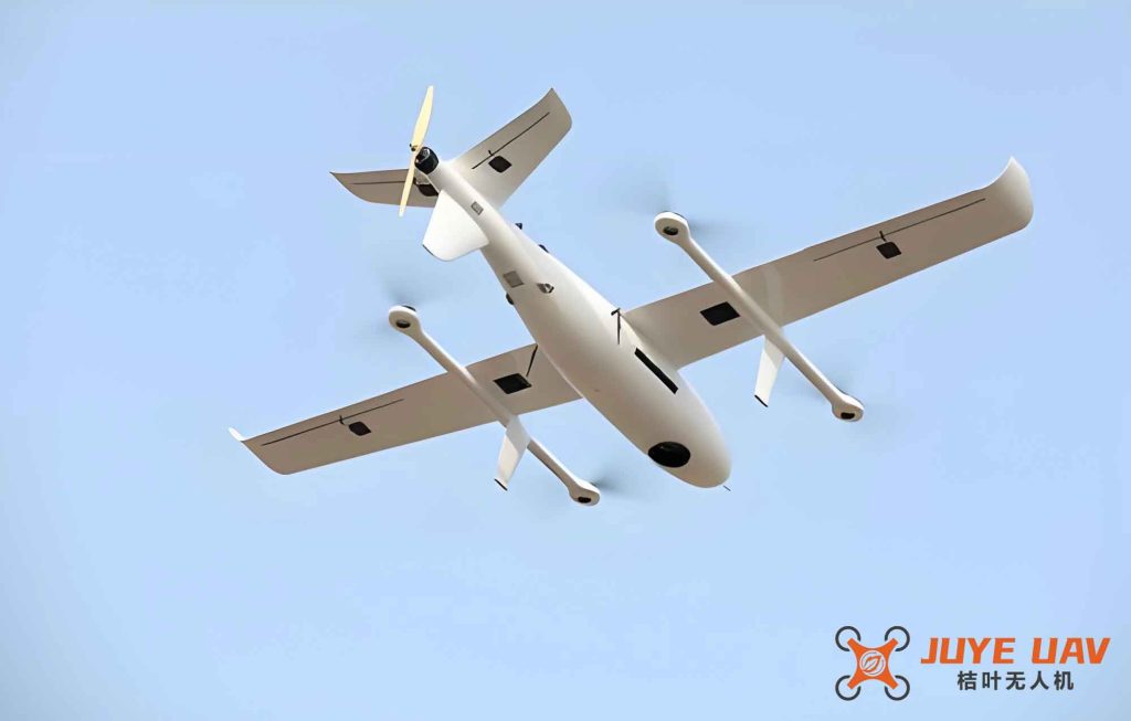
We address the challenges of formation assembly efficiency and geometric precision for small fixed-wing UAV swarms. By integrating a Dubins-based loose formation rapid assembly strategy with a distributed consensus-based fine formation control method, we achieve fast and efficient aggregation, stable formation maintenance, and smooth formation transformations.
The following sections detail our modeling, algorithm design, and simulation validation.
1. Problem Description and Control Architecture
We consider multiple small fixed-wing UAVs launched sequentially from a same ground platform with a constant time interval. After climbing to a designated altitude, each UAV flies at a constant cruising speed within a limited speed range. We assume ideal communication (no delay, no interference) and no wind disturbance. Each UAV is treated as a mass point in a 2D plane after altitude stabilization. The formation control problem is divided into two stages:
- Loose assembly stage: Using Dubins path planning to quickly bring all UAVs to a common rendezvous point with near‑identical velocity vectors, while avoiding collisions.
- Fine formation stage: Switching to a distributed consensus controller based on a virtual leader to achieve precise geometric configuration and maintain the shape during subsequent maneuvers.
This hierarchical strategy combines the fast convergence of geometric path planning with the high‑accuracy tracking ability of consensus algorithms.
2. Modeling and Algorithms
2.1 Fixed-Wing UAV Kinematic Model
For simplicity, we adopt a 2D point‑mass model under coordinated turn assumptions. The state of UAV \(i\) is described by its position \((x_i, y_i)\), ground speed \(V_{gi}\), and heading angle \(\chi_i\). The kinematic equations are:
$$
\dot{x}_i = V_{gi} \cos \chi_i, \quad
\dot{y}_i = V_{gi} \sin \chi_i, \quad
\dot{\chi}_i = \frac{a_i}{V_{gi}},
$$
where \(a_i\) is the lateral acceleration bounded by \(a_{\max,i}\). The speed is also bounded: \(V_{\min,i} \le V_{gi} \le V_{\max,i}\). The minimum turn radius is \(r_{\min,i}= V_{gi}^2 / a_{\max,i}\). These constraints are critical for the Dubins path generation.
2.2 Dubins Path Planning for Rapid Assembly
We assume all UAVs start at the same origin \((0,0)\) with identical initial heading \(\pi/2\), but at different launch times \(t_i = (i-1)\Delta t\). The desired terminal states (position and heading) for each UAV are set to achieve a specific formation pattern. We use a CLC (circle‑line‑circle) Dubins path type, where each UAV performs two turns of radius \(r_{i1}, r_{i2}\) (both equal to \(r_{\min}\)) and a straight segment. The path length must satisfy:
$$
\begin{aligned}
& r_{i1}\phi_{i1} + d_i + r_{i2}\phi_{i2} = V_g (t_i + \Delta t_{\text{ref}}) \\
& \begin{cases}
x_i = r_{i1}(1-\cos\phi_{i1}) + d_i \sin\phi_{i1} + r_{i2}(\cos\phi_{i2}-\cos(\phi_{i1}+\phi_{i2})) \\
y_i = r_{i1}\sin\phi_{i1} + d_i \cos\phi_{i1} + r_{i2}(\sin\phi_{i2}+\sin(\phi_{i1}+\phi_{i2}))
\end{cases}
\end{aligned}
$$
where \(\phi_{i1}, \phi_{i2}\) are the turn angles, \(d_i\) is the straight segment length, and \(\Delta t_{\text{ref}}\) is the reference time for the first UAV. The unknowns form a nonlinear system. We solve it using two approaches:
| Method | Approach | Pros | Cons |
|---|---|---|---|
| Analytical | Pick one UAV as reference, fix its variables, solve the remaining equations exactly by searching over a discrete set of angles. | Provides the true shortest assembly time; high precision. | Computationally expensive for online use; requires offline pre‑computation. |
| Genetic Algorithm (GA) | Minimize an objective function \(F = \sum_i (l_{si}^2 + l_{xi}^2 + l_{yi}^2)\) subject to constraints, using GA to search for suboptimal solution. | Fast; can be executed quasi‑real‑time; flexible for different initial conditions. | Only suboptimal solution; residual position errors up to 10 m. |
We explicitly check collision avoidance by ensuring inter‑UAV distances never drop below a safety threshold (25 m). If a candidate path violates this, it is discarded. The flowchart of the GA‑based planner is as follows:
- Initialize population with random parameter vectors.
- Evaluate fitness (total path length + penalty for collisions).
- Selection, crossover, mutation.
- Return the best feasible path after a fixed number of generations.
2.3 Consensus‑Based Fine Formation Control
After the loose assembly (all UAVs arrive near the desired point with similar speeds), we switch to a distributed consensus law. We model the communication topology as an undirected graph where each UAV can receive state information from the virtual leader (index 0) and from its neighbors. The second‑order consensus control for UAV \(i\) is:
$$
\begin{aligned}
u_i = &-\alpha\left[(\xi_i – \xi_0 – d_i) + \beta(\zeta_i – \zeta_0)\right] \\
&-\sum_{j=1}^{n} a_{ij}\left[(\xi_i – \xi_j – (d_i – d_j)) + \beta(\zeta_i – \zeta_j)\right],
\end{aligned}
$$
where:
- \(\xi_i = [x_i, y_i]^T\), \(\zeta_i = [\dot{x}_i, \dot{y}_i]^T\).
- \(d_i\) is the desired relative position w.r.t. the leader (e.g., for a diagonal line, \(d_i = [\Delta x_i, \Delta y_i]\)).
- \(\alpha>0\) is the leader‑follower gain (we set \(\alpha=1\)).
- \(\beta>0\) is the velocity consensus gain (\(\beta=2\)).
- \(a_{ij}\) are adjacency weights (0 or 1 for all neighbors).
The virtual leader moves with constant velocity \(\zeta_0 = [V_g, 0]^T\). The control law ensures that all UAVs converge to the desired relative positions exponentially. For formation transition (e.g., from oblique line to V‑shape), we change \(d_i\) to the new formation vectors; the controller automatically guides the transition while keeping a safe inter‑vehicle distance.
3. Simulation and Results
We simulate three small fixed‑wing UAVs with the parameters listed below.
| Parameter | Value |
|---|---|
| Minimum speed | 35 m/s |
| Maximum speed | 45 m/s |
| Cruising speed | 40 m/s |
| Maximum lateral acceleration | 0.5 m/s² |
| Minimum turn radius | 200 m |
| Launch time interval | 2 s |
| Desired inter‑UAV separation (x and y) | 100 m each |
| Safety distance | 25 m |
For the Dubins assembly, we compare analytical and GA results:
| UAV | Analytical \(\phi\) (rad) | Analytical \(d\) (m) | GA \(\phi\) (rad) | GA \(d\) (m) |
|---|---|---|---|---|
| 1 | 1.745 | 300.0 | 1.67 | 452 |
| 2 | 1.579 | 217.6 | 1.58 | 412 |
| 3 | 1.116 | 363.0 | 1.43 | 453 |
| Assembly time: Analytical: 24.95 s; GA: 63.8 s (suboptimal but collision‑free) | ||||
After loose assembly, we apply the consensus controller. Starting from the residual errors (up to 10 m position and 2 m/s speed mismatch), the formation converges to a stable oblique line within approximately 10 s (position error < 1 mm). Then we command a transition to a V‑shape (equilateral triangle with side 100 m). The controller smoothly guides the transition, reaching the new formation in about 350 s while maintaining inter‑UAV distances always above 25 m. The minimum distance during the transition is shown in the simulation, confirming safe operation.
4. Conclusion
We have presented a two‑stage formation control framework for small fixed‑wing UAV swarms launched sequentially. The first stage uses Dubins path planning (with either analytical or GA‑based optimization) to achieve rapid loose assembly. The second stage employs a distributed consensus algorithm based on a virtual leader to refine the formation into a precise geometric pattern and to perform shape transitions. Simulation results validate that the method effectively reduces assembly time, maintains stable geometry, and ensures collision avoidance. Future work will incorporate communication delays, dynamic obstacles, and tighter aerodynamic coupling for close formation flight.