
In recent years, unmanned aerial vehicle (UAV) technology has matured considerably, leading to the extension of UAS (Unmanned Aerial System) applications from military to civilian domains. In disaster scenarios causing large-scale communication outages, medium-sized fixed-wing UAVs can fly rapidly to designated positions and carry emergency airborne equipment to provide wireless network coverage to the ground. Studying the air-to-ground channel model and its characteristics in such emergency situations is crucial for the design and optimization of UAS communication systems. In 2017, the 3rd Generation Partnership Project (3GPP) initiated research on LTE aerial channels and developed several protocol specifications, but these only focus on low-altitude (below 300 m) wireless communication for terrestrial mobile terminals. Traditional channel models such as Okumura-Hata and UMa are also only applicable to ground scenarios. Akram Al-Hourani et al. studied an air-to-ground path loss model for urban environments, but that model is only valid for static base station transmission and is not suitable for medium- to low-altitude, high-dynamic fixed-wing UAV emergency scenarios.
All the above models target low-altitude small UAV air-to-ground channels and do not apply to medium- to high-altitude, high-dynamic medium- to large-sized fixed-wing UAV emergency scenarios. Moreover, these models are based on traditional empirical approaches, which suffer from low applicability and accuracy in real-world deployments. In this work, we propose a novel air-to-ground intelligent wireless propagation model based on the XGBoost algorithm for medium-sized fixed-wing UAV emergency scenarios. By extracting features from engineering parameters collected by the airborne base station, we innovatively incorporate dynamic 3D antenna gain values to enhance prediction accuracy. We compare our model with the traditional air-to-ground channel model and the channel model specified in the 3GPP TR 36.777 protocol. Results demonstrate that the XGBoost-based path loss model achieves significantly higher prediction accuracy than conventional wireless propagation models.
System Setup and Feature Preprocessing
System Setup
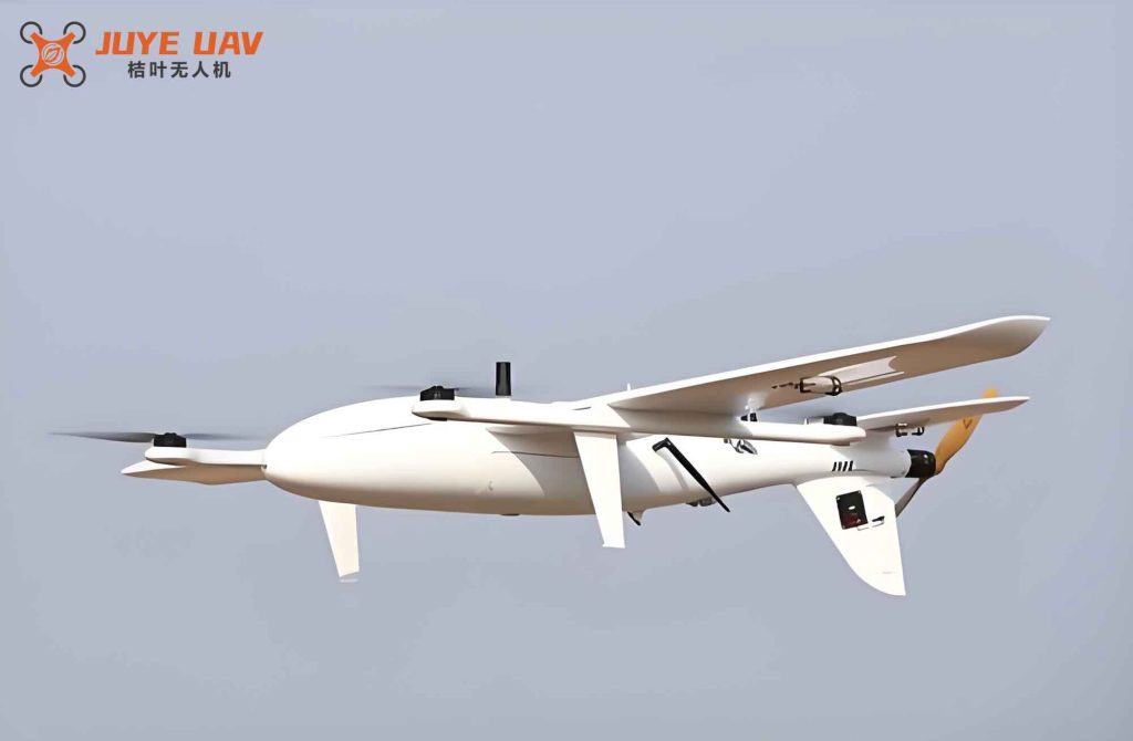
The experiments were conducted at open test sites. The ground receiving terminal was placed approximately 1 m above the ground. An airborne fixed-wing UAV carried a base station and an antenna to transmit signals at a frequency of 900 MHz. The ground terminal recorded the received signal strength and its own position. The UAV’s position information and attitude data were stored onboard and later processed. The test equipment architecture is depicted in the figure below. The fixed-wing UAV used in the tests is a medium-sized model, and the environment was an open area with minimal obstacles.
The test base station operated in the LTE FDD 900 MHz band. The 900 MHz band offers strong diffraction capability in free space and is less affected by fading. The airborne antenna has an operating frequency range from 820 MHz to 960 MHz, with a maximum gain of 3 dBi. The antenna was suspended beneath the wing, aligned to the center of the flight circle to achieve continuous coverage. During tests, the fixed-wing UAV circled clockwise around a fixed center with a radius of 300 m. The UAV flew at three different altitudes: 500 m, 1000 m, and 1500 m. Test personnel walked from the circle center outward, conducting fixed-point and drive tests every 0.5 km.
Feature Construction
The dataset includes 12 raw features, such as UAV (base station) position, terminal position, transmit power, and UAV flight attitude. We collected 8,000 data samples. After preprocessing, we constructed seven additional geometric and angular features, as summarized in Table 1.
| Feature Type | Raw Features | Constructed Features | Unit |
|---|---|---|---|
| Geometric | Terminal longitude \(A_j\) | Horizontal distance \(d_{2D}\) | m |
| Terminal latitude \(A_w\) | 3D distance \(d_{3D}\) | m | |
| UAV longitude \(B_j\) | Height difference \(H_d\) | m | |
| Angular | UAV latitude \(B_w\) | Azimuth angle \(\phi_{ue}\) | rad |
| Terminal height \(H_{ue}\) | Elevation angle \(\theta_{ue}\) | rad | |
| UAV flight height \(H_{uav}\) | Terminal-antenna azimuth \(\phi\) | rad | |
| Attitude | UAV speed \(V_{uav}\) | Terminal-antenna elevation \(\theta\) | rad |
| UAV heading \(\phi_{uav}\) | |||
| Installed | UAV roll \(\theta_{uav}\) | ||
| Channel | Transmit power \(P_{Tx}\) | MHz | |
| Carrier frequency \(f_c\) | MHz | ||
| 3D antenna gain \(G_{Tx3D}\) | dBi |
In conventional models, the predicted variable is path loss, but in practice the more intuitive measurement is the received signal power, i.e., RSRP (Reference Signal Receiving Power). Based on the TD-LTE link budget model, the measured path loss \(PL\) is computed as:
$$
PL = P_{Tx} + G_{Tx3D} + G_{rx} – P_{Rx}
$$
where \(G_{Tx3D}\) is the dynamic 3D transmit antenna gain, \(P_{Tx}\) is the base station cell transmit power, \(G_{rx}\) is the receive antenna gain, and \(P_{Rx}\) is the measured received power.
Distance and Angle Feature Construction
Let the horizontal distance between the UAV base station and the ground terminal be \(d_{2D}\). Point A represents the ground terminal, point B the UAV, and R the Earth’s mean radius. \(A_j, A_w\) denote the longitude and latitude of the terminal, and \(B_j, B_w\) denote those of the UAV. The angle \(c\) subtended by the arc AB is derived from the spherical cosine law:
$$
c = \arccos\bigl(\cos(90^\circ – B_w)\cos(90^\circ – A_w) + \sin(90^\circ – B_w)\sin(90^\circ – A_w)\cos(B_j – A_j)\bigr)
$$
Converting to radians and then computing distances:
$$
c(\text{rad}) = c \cdot \frac{\pi}{180}
$$
$$
d_{2D} = R \cdot c
$$
$$
d_{3D} = \sqrt{d_{2D}^2 + (H_{uav} – H_{ue})^2}
$$
The terminal’s azimuth angle relative to the UAV, \(\phi_{ue}\), is measured clockwise from true north:
$$
\phi_{ue} = \arctan\left( \frac{(B_j – A_j)\cos B_w}{B_w – A_w} \right)
$$
The elevation angle \(\theta_{ue}\) (angle between the line connecting terminal and UAV and the horizontal plane) is:
$$
\theta_{ue} = \arctan\left( \frac{d_{2D}}{H_{uav} – H_{ue}} \right)
$$
Dynamic 3D Antenna Gain Construction
In real measurements, the positions of the terminal and fixed-wing UAV change dynamically, so the antenna gain at each point is not a constant but a dynamic 3D value. We innovatively incorporate this dynamic 3D antenna gain into the air-to-ground propagation model to reduce the error caused by assuming constant gain. The antenna gain is simulated using interpolation based on the measured horizontal and vertical radiation patterns. The interpolation formula is:
$$
Gain(\Phi_s, \theta_s) = H(\Phi_s) – \left[ \frac{\pi – |\Phi_s|}{\pi} (H(0) – V(\theta_s)) + \frac{|\Phi_s|}{\pi} (H(\pi) – V(\pi – \theta_s)) \right]
$$
Here, \(\Phi_s\) is the horizontal angle of the terminal in the UAV coordinate system, \(\theta_s\) is the elevation angle, \(H(\Phi_s)\) is the horizontal gain, and \(V(\theta_s)\) is the vertical gain. The azimuth \(\phi\) and elevation \(\theta\) of the terminal relative to the 3D antenna are computed by taking the difference between the terminal’s relative angles and the UAV’s roll (\(\phi_{uav}\)) and heading (\(\theta_{uav}\)) modulo \(2\pi\):
$$
\phi = (\phi_{ue} – \phi_{uav}) \mod (2\pi)
$$
$$
\theta = (\theta_{ue} – \theta_{uav}) \mod (2\pi)
$$
Using the simulated 3D antenna pattern, we obtain the dynamic 3D gain \(G_{Tx3D}\) for each sample, which is then substituted into the link budget equation to derive the path loss \(PL\) for model training.
Feature Extraction
To evaluate the impact of each feature on path loss, we compute the Pearson correlation coefficient \(\rho_{XY}\) between each feature and the path loss \(PL\):
$$
\rho_{XY} = \frac{\text{cov}(X,Y)}{\sigma_X \sigma_Y} = \frac{E[(X-\mu_X)(Y-\mu_Y)]}{\sigma_X \sigma_Y}
$$
The results are sorted by absolute correlation value in descending order in Table 2.
| Rank | Feature | Correlation Coefficient | Absolute Value |
|---|---|---|---|
| 1 | \(d_{3D}\) | 0.29 | 0.29 |
| 2 | \(d_{2D}\) | 0.28 | 0.28 |
| 3 | \(\theta_{ue}\) | -0.28 | 0.28 |
| 4 | \(\theta_{uav}\) | -0.26 | 0.26 |
| 5 | \(\phi_{ue}\) | 0.21 | 0.21 |
| 6 | \(V_{uav}\) | -0.20 | 0.20 |
| 7 | \(\phi_{uav}\) | 0.18 | 0.18 |
| 8 | \(H_d\) | -0.13 | 0.13 |
The results show that path loss is most strongly correlated with the 3D distance \(d_{3D}\) and horizontal distance \(d_{2D}\) (positive correlation), as well as with angles \(\theta_{ue}\), \(\theta_{uav}\), and \(\phi_{ue}\). Hence, we select the five most relevant features \(\{d_{3D}, d_{2D}, \theta_{ue}, \theta_{uav}, \phi_{ue}\}\) as input variables for model construction.
Classical Path Loss Model Adaptation
Evaluation Metrics
We use the Root Mean Square Error (RMSE) and Mean Error (ME) to evaluate model performance. For \(n\) samples:
$$
RMSE = \sqrt{\frac{1}{n} \sum_{i=1}^{n} (\hat{y}_i – y_i)^2}
$$
$$
ME = \frac{1}{n} \sum_{i=1}^{n} (\hat{y}_i – y_i)
$$
where \(\hat{y}_i\) is the predicted path loss and \(y_i\) is the measured path loss for the \(i\)-th sample. Lower errors indicate better predictive performance.
3GPP Model (RMa-AV LOS)
The 3GPP TR 36.777 protocol defines a low-altitude air-to-ground propagation model (RMa-AV LOS) for altitudes below 300 m. The model is expressed as:
$$
PL_{\text{3GPP}}^{\text{RMa-AV-LOS}}(f_c, d_{3D}) = \max\bigl(23.9 – 1.8 \log_{10}(H_{uav}), 20\bigr) \log_{10}(d_{3D}) + 20 \log_{10}\left(\frac{40\pi f_c}{3}\right)
$$
The applicable conditions are:
$$
\begin{cases}
10\,\text{m} \le H_{uav} \le 300\,\text{m}\\
d_{2D} \le 10\,\text{km}
\end{cases}
$$
For medium- to high-altitude scenarios (above 300 m), this model essentially reduces to free-space path loss:
$$
PL = 20 \log_{10}(d) + 20 \log_{10}(f) + 20 \log_{10}\left(\frac{4\pi}{c}\right)
$$
A2G Model (Akram Al-Hourani)
This model considers the line-of-sight (LOS) probability in air-to-ground transmission. The total path loss is the weighted sum of LOS and NLOS losses:
$$
PL_{\text{LOS}} = 20 \log_{10}(d) + 20 \log_{10}(f) + 20 \log_{10}\left(\frac{4\pi}{c}\right) + \eta_{\text{LOS}}
$$
$$
PL_{\text{NLOS}} = 20 \log_{10}(d) + 20 \log_{10}(f) + 20 \log_{10}\left(\frac{4\pi}{c}\right) + \eta_{\text{NLOS}}
$$
The average path loss is:
$$
PL = P_{\text{LOS}} \cdot PL_{\text{LOS}} + P_{\text{NLOS}} \cdot PL_{\text{NLOS}}
$$
The LOS probability is modeled as:
$$
P_{\text{LOS}} = \frac{1}{1 + a e^{-b\left(\frac{180}{\pi} \theta – a\right)}}
$$
where \(a\) and \(b\) are environment-dependent parameters, and \(\theta\) is the elevation angle. Substituting, the final expression becomes:
$$
PL = \frac{\eta_{\text{LOS}} – \eta_{\text{NLOS}}}{1 + a e^{-b(\theta – a)}} + 20 \log_{10}(d) + 20 \log_{10}(f) + 20 \log_{10}\left(\frac{4\pi}{c}\right) + \eta_{\text{NLOS}}
$$
In our open-area test environment, we set the excess losses \(\eta_{\text{LOS}} = 1\) dB and \(\eta_{\text{NLOS}} = 20\) dB, and environment parameters \(a = 11.95\), \(b = 0.136\).
XGBoost-Based Wireless Channel Model
XGBoost (eXtreme Gradient Boosting) is a highly efficient and scalable machine learning algorithm developed by Chen et al. It achieves superior prediction accuracy compared to many other algorithms. We adopt XGBoost as the core algorithm for path loss regression in high‑dynamic fixed‑wing UAV emergency scenarios. The algorithm is briefly described as follows.
Regularized Loss Function
Let \( \hat{y}_i \) be the predicted path loss and \(y_i\) the measured value for sample \(i\). The regularized loss function is:
$$
\mathcal{L} = \sum_{i=1}^{n} l(\hat{y}_i, y_i) + \sum_{k=1}^{T} \Omega(f_k)
$$
where \(\Omega(f) = \gamma T + \frac{1}{2}\lambda \sum_{j=1}^{T} \omega_j^2\), with \(T\) being the number of leaves and \(\omega_j\) the leaf weights. The base learner is a regression tree \(f_t(x) = w_{q(x)}\), where \(q(x)\) maps an input to a leaf index.
Objective Optimization
At the \(t\)-th iteration, the model is updated by adding the new tree \(f_t\). The objective becomes:
$$
\mathcal{L}^{(t)} = \sum_{i=1}^{n} l\bigl(y_i, \hat{y}_i^{(t-1)} + f_t(x_i)\bigr) + \sum_{k=1}^{t-1} \Omega(f_k) + \Omega(f_t)
$$
Using a second-order Taylor expansion:
$$
\mathcal{L}^{(t)} \approx \sum_{i=1}^{n} \left[ l(y_i,\hat{y}_i^{(t-1)}) + g_i f_t(x_i) + \frac{1}{2} h_i f_t^2(x_i) \right] + \Omega(f_t)
$$
where \(g_i = \partial_{\hat{y}^{(t-1)}} l(y_i, \hat{y}_i^{(t-1)})\) and \(h_i = \partial^2_{\hat{y}^{(t-1)}} l(y_i, \hat{y}_i^{(t-1)})\). Removing constant terms and substituting \(f_t\) and \(\Omega\):
$$
\mathcal{L}^{(t)} \approx \sum_{i=1}^{n} \left[ g_i w_{q(x_i)} + \frac{1}{2} h_i w_{q(x_i)}^2 \right] + \gamma T + \frac{1}{2}\lambda \sum_{j=1}^{T} w_j^2
$$
Grouping samples by leaf indices \(I_j = \{i | q(x_i)=j\}\) yields:
$$
\mathcal{L}^{(t)} = \sum_{j=1}^{T} \left[ \left(\sum_{i \in I_j} g_i\right) w_j + \frac{1}{2}\left(\sum_{i \in I_j} h_i + \lambda\right) w_j^2 \right] + \gamma T
$$
For a fixed tree structure, the optimal leaf weight \(w_j^*\) is obtained by setting the derivative to zero:
$$
w_j^* = -\frac{G_j}{H_j + \lambda}, \quad G_j = \sum_{i \in I_j} g_i, \quad H_j = \sum_{i \in I_j} h_i
$$
The minimal loss after substituting \(w_j^*\) is:
$$
\mathcal{L}^* = -\frac{1}{2} \sum_{j=1}^{T} \frac{G_j^2}{H_j + \lambda} + \gamma T
$$
Tree Splitting Criterion
When splitting a leaf node, the algorithm evaluates all possible splits on all features and selects the one that maximizes the gain:
$$
\text{Gain} = \frac{1}{2} \left[ \frac{G_L^2}{H_L + \lambda} + \frac{G_R^2}{H_R + \lambda} – \frac{(G_L + G_R)^2}{(H_L + H_R) + \lambda} \right] – \gamma
$$
The greedy split algorithm iterates over each feature (our five selected features) and each possible split point, computing the gain. The split with the highest gain is chosen. The pseudocode for the precise greedy algorithm is given in Table 3.
| Algorithm: Exact Greedy Splitting |
|---|
| Input: Current node dataset \(I = \{(d_{3D}, d_{2D}, \theta_{ue}, \theta_{uav}, \phi_{ue}), PL\}\) |
| Input: Feature dimension \(m = 5\) |
| \(gain \leftarrow 0\) \(G = \sum_{i \in I} g_i\), \(H = \sum_{i \in I} h_i\) |
| for \(k = 1\) to \(m\) do: \(G_L \leftarrow 0\), \(H_L \leftarrow 0\) for each sorted element \(j\) in \(I\) by \(x_{jk}\): \(G_L \leftarrow G_L + g_j\), \(H_L \leftarrow H_L + h_j\) \(G_R = G – G_L\), \(H_R = H – H_L\) \(Score \leftarrow \frac{G_L^2}{H_L+\lambda} + \frac{G_R^2}{H_R+\lambda} – \frac{G^2}{H+\lambda}\) \(gain \leftarrow \max(gain, Score)\) |
| Output: Maximum gain and corresponding split feature/value |
Hyperparameter Tuning
We optimize the XGBoost model using grid search. The final optimized parameters are listed in Table 4.
| Parameter | Value |
|---|---|
| Max depth | 6 |
| Learning rate | 0.1 |
| Number of estimators | 1000 |
| Booster | gbtree |
| Gamma | 0 |
| Lambda | 3 |
| Objective | logistic |
| Subsample ratio | 0.7 |
Experimental Results and Analysis
To validate the prediction accuracy of the XGBoost-based intelligent propagation model, we compare it with the classical 3GPP RMa-AV LOS model and the A2G model. All three models are trained and tested on the same datasets collected from two open test sites. Fixed-wing UAV flights were performed in circling patterns, and data were collected for both fixed-point and drive test scenarios.
The following figures illustrate the prediction performance for one test location. (Note: Due to the text-only format, we describe the trends rather than displaying figures.) The path loss variation with UAV circling shows that the received path loss fluctuates with the fixed-wing UAV’s attitude, with a maximum fluctuation range of about 20 dB. The temporal evolution of path loss follows a quasi-sinusoidal pattern. The XGBoost model closely follows this pattern, while the classical models only capture the mean trend. As distance increases, path loss increases. For near distances (large elevation angles), the A2G model’s LOS probability approaches 100%, making it similar to the free-space 3GPP model. At far distances (around 5 km), the A2G model deviates from free-space loss because of the increasing NLOS probability. Nevertheless, both classical models yield large errors compared to the XGBoost model. The cumulative distribution function (CDF) of RSRP also shows that the XGBoost model’s curve matches the measured data best.
We summarize the numerical errors in Table 5.
| Test Location | Model | RMSE (dB) | ME (dB) |
|---|---|---|---|
| Site A | 3GPP | 10.60 | 12.93 |
| A2G | 10.28 | 12.77 | |
| XGBoost | 3.64 | -0.80 | |
| Site B | 3GPP | 7.86 | 9.95 |
| A2G | 7.20 | 9.23 | |
| XGBoost | 4.99 | -0.15 |
From Table 5, the XGBoost model achieves the lowest RMSE and ME at both test sites. At Site A, the RMSE of XGBoost is 3.64 dB, which is a 6.96 dB improvement over the 3GPP model, and the ME improves by 12.13 dB. At Site B, the XGBoost model also outperforms the others, with an RMSE of 4.99 dB and an ME of -0.15 dB. These values satisfy the typical requirement that the RMSE of a usable propagation model should be less than 8 dB. Moreover, while classical models only fit the general trend of path loss variation, the XGBoost model captures the point‑wise fluctuations caused by the fixed-wing UAV’s dynamic attitude during circling, making it much more suitable for high‑dynamic emergency scenarios.
Conclusion
We have developed an air-to-ground intelligent wireless propagation model for medium‑ to high‑altitude, high‑dynamic fixed-wing UAV emergency scenarios based on the XGBoost algorithm. The model innovatively incorporates dynamic 3D antenna gain values to improve accuracy. Comparisons with the classical 3GPP RMa-AV LOS model and the A2G model demonstrate that the XGBoost model provides the best prediction accuracy, with RMSE below 4.99 dB and mean error within ±0.8 dB. This accurate prediction of air‑to‑ground path loss for fixed-wing UAV operations is of great significance for the design and optimization of emergency communication systems.