
In modern civil and military operations, the application of fixed-wing drones in swarm or formation scenarios has gained increasing attention due to their superior endurance, payload capacity, and aerodynamic efficiency compared to rotary-wing platforms. However, controlling a group of fixed-wing drones to maintain a prescribed formation geometry under dynamic maneuvers remains a challenging problem, especially when the drones are modeled with six degrees of freedom (6-DoF) and realistic flight dynamics. Traditional control methods, such as PID controllers, often require tedious manual tuning and struggle with the strong coupling between multiple control surfaces. In this paper, we present our novel hierarchical deep reinforcement learning framework named Hierarchical Guidance and Control Proximal Policy Optimization (HGC-PPO), which is specifically designed for the formation control of 6-DoF fixed-wing drones. Our approach decomposes the complex formation control problem into two distinct layers: a guidance layer and a control layer. The guidance layer, inspired by the leader-follower paradigm, generates high-level commands such as desired velocity, roll angle, and altitude. The control layer, realized by a multi-input multi-output (MIMO) neural network, directly maps the state information to the four control surface deflections (aileron, elevator, rudder, and throttle). To facilitate efficient learning, we incorporate a curriculum learning strategy into the reward function of the guidance layer, which gradually increases the task difficulty and smooths the learning curve. Extensive simulation results demonstrate that our HGC-PPO algorithm achieves stable, accurate, and efficient formation control for fixed-wing drones, outperforming baseline methods such as standard PPO and PID-based hybrid approaches.
Throughout this paper, we emphasize the unique challenges and solutions associated with fixed-wing drones. Unlike quadrotors, fixed-wing drones cannot hover and must maintain a minimum forward speed to generate lift, which imposes additional constraints on formation control. Our HGC-PPO framework explicitly accounts for these constraints through appropriate state normalization, action clipping, and termination conditions. The remainder of this article is organized as follows. First, we describe the 6-DoF flight dynamics model used for our fixed-wing drones. Then, we present the overall HGC-PPO architecture and detail the design of both the control layer and the guidance layer. Next, we provide extensive experimental validation, including training curves, ablation studies, and multi-drone formation flights under various maneuvers. Finally, we conclude with a summary of our contributions and future directions.
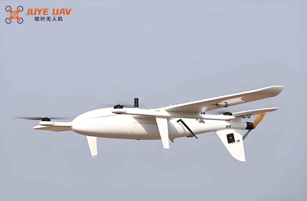
Before diving into the methodology, we present a conceptual illustration of fixed-wing drones in formation flight.
1. Flight Dynamics Modeling of Fixed-Wing Drones
We model each fixed-wing drone as a rigid body with six degrees of freedom. The equations of motion are derived from Newton-Euler formalism and are integrated using the open-source flight dynamics simulator JSBSim. The state of a fixed-wing drone is described by its position in the inertial frame, its velocity components in the body frame, and its Euler angles (roll φ, pitch θ, yaw ψ). The control inputs are the deflections of the aileron (δa), elevator (δe), rudder (δr), and throttle (δt). The kinematic relations between the body angular rates (p, q, r) and the Euler angle rates are given by:
$$
\begin{aligned}
\dot{\phi} &= p + q \sin\phi \tan\theta + r \cos\phi \tan\theta \\
\dot{\theta} &= q \cos\phi – r \sin\phi \\
\dot{\psi} &= (q \sin\phi + r \cos\phi) / \cos\theta
\end{aligned}
$$
The velocity components in the body frame (u, v, w) are related to the airspeed V, angle of attack α, and sideslip angle β through:
$$
\begin{aligned}
u &= V \cos\alpha \cos\beta \\
v &= V \sin\beta \\
w &= V \sin\alpha \cos\beta
\end{aligned}
$$
The aerodynamic forces and moments are computed using a lookup-table model for a generic fixed-wing drone. The model includes nonlinear effects such as stall and control surface effectiveness variations with airspeed. The simulation time step is fixed at 0.2 s, which provides a good balance between accuracy and computational efficiency for reinforcement learning training.
To ensure the fidelity of our dynamics model, we validated it against known flight test data of small fixed-wing drones. The model captures the essential coupling between longitudinal and lateral motions, which is critical for formation control. For example, a change in throttle affects not only forward speed but also pitch attitude due to the thrust moment arm. Similarly, aileron deflection induces adverse yaw, requiring coordinated rudder input. Traditional PID controllers that treat each channel independently often fail to achieve good performance in such coupled systems. This motivates our use of a learning-based MIMO controller.
2. HGC-PPO Algorithm
2.1 Overall Architecture
Our HGC-PPO algorithm is built upon the Proximal Policy Optimization (PPO) framework but extends it with a hierarchical structure. The key idea is to split the formation control task into two sub-tasks:
- Guidance Layer: It receives the relative state between the leader (or desired formation point) and the follower fixed-wing drone, and outputs high-level commands: desired velocity vt (80–200 m/s), desired roll angle φt (–72° to 72°), and desired altitude zt (1500–9000 m).
- Control Layer: It takes the current state of the fixed-wing drone and the guidance commands, and outputs the four control surface deflections (δa, δe, δr, δt) directly. This layer is trained separately first, then frozen during guidance layer training, or they can be trained sequentially.
This decomposition significantly reduces the state space dimensionality for each layer, making the learning problem more tractable. The control layer learns to track arbitrary step commands in velocity, roll, and altitude, while the guidance layer learns to issue those commands such that the overall formation error is minimized. The two layers are connected through the intermediate command variables, which serve as a natural interface.
The overall optimization objective for the formation is to minimize the aggregate position error of all followers relative to their desired positions expressed in the leader’s body frame. Let pi be the actual relative position of follower i and pides be the desired relative position. The cost function J is:
$$
J = \min \sum_{t=1}^{T} \sum_{i=1}^{N} \| \mathbf{p}_i(t) – \mathbf{p}_i^{\text{des}}(t) \|_2
$$
In our experiments, we consider a formation of five fixed-wing drones: one leader and four followers arranged in a diamond or line pattern with a separation of 80 m between adjacent drones. The leader follows a predefined trajectory (straight, turning, S-turn, spiral) while the followers attempt to maintain the formation using our HGC-PPO controller. We assume perfect communication with negligible delay and no external disturbances to isolate the control performance.
2.2 Control Layer Design
The control layer is a neural network with two hidden layers of 256 units each, using Tanh activation. The state space for the control layer includes:
- Body velocity components: u, v, w (normalized)
- Command tracking errors: Δz = zt – z, Δvc = vt – vc, Δφ = φt – φ
- Current roll angle φ
The action space is the four control deflections δa, δe, δr ∈ [–1, 1] and throttle δt ∈ [0.2, 1]. The lower bound on throttle prevents stall. The reward function for the control layer consists of two parts: an error reward and a stability reward.
The error reward rerror is defined as the geometric mean of exponential functions of squared errors:
$$
r_{\text{error}} = \sqrt[n]{\prod_{i=1}^{n} e^{-k_i ( \text{target}_i – \text{value}_i )^2 }}
$$
where n = 3 (height, velocity, roll) and ki are scaling coefficients to balance the different units. The stability reward penalizes large changes in control inputs:
$$
r_{\text{stable}} = \sqrt[n]{\prod_{i=1}^{n} e^{-k_i (\Delta \text{in}_i)^2 }}
$$
where Δini is the change in each control surface deflection from the previous time step. The total reward is r = rerror + rstable.
We also implement termination conditions to avoid dangerous states and speed up training:
| Condition | Threshold | Penalty r |
|---|---|---|
| Roll tracking error |Δφ| > 45° | 45° | –5 |
| Velocity tracking error |Δvc| > 80 m/s | 80 m/s | –5 |
| Altitude tracking error |Δz| > 1500 m | 1500 m | –5 |
| Normal acceleration |an| > 2.5 g | 2.5 g | –5 |
| Tangential acceleration |at| > 0.5 g | 0.5 g | –5 |
| Roll rate |p| > 40°/s | 40°/s | –5 |
| Pitch rate |q| > 5°/s | 5°/s | –5 |
| Yaw rate |r| > 4°/s | 4°/s | –5 |
| Maximum episode length exceeded | 200 s (1000 steps) | +5 |
We train the control layer for 300 update iterations with a batch size of 15 episodes per update. The hyperparameters used are summarized in Table 2.
| Parameter | Value |
|---|---|
| Discount factor γ | 0.99 |
| Optimizer | Adam |
| Learning rate | 0.002 |
| Number of steps per episode | 1000 (200 s) |
| Batch size (episodes per update) | 15 |
| Entropy coefficient | 0.01 |
| PPO clip range | 0.2 |
| GAE lambda | 0.98 |
| Simulation time step | 0.2 s |
| Activation function | Tanh |
| Actor network layers | [256, 256, 256] |
| Critic network layers | [256, 256, 256] |
2.3 Guidance Layer Design with Curriculum Learning
The guidance layer is also a neural network with the same architecture as the control layer (two hidden layers of 256 Tanh units). The state vector for the guidance layer is more comprehensive, including the relative position (Δx, Δy, Δz), the distance in the horizontal plane ρ, the speed difference Δvc, the angle between velocity direction and distance vector η, the heading errors (ψt – ψ, ψ̇t – ψ̇), and the body velocities (u, v, w) as well as Euler angles (φ, ψ, θ). The action space consists of the three guidance commands: desired velocity vt, desired roll φt, and desired altitude zt.
The reward function for the guidance layer is a weighted sum of several components, with one of the weights being dynamic according to a curriculum learning schedule. The total reward at time t is:
$$
r_t = k(r) \, r_{t,\text{dis}} + \lambda_1 r_{t,z} + \lambda_2 r_{t,\phi} + \lambda_3 r_{t,v}
$$
where rt,dis penalizes the horizontal distance error, rt,z penalizes the altitude error, rt,ϕ is a roll guidance reward, and rt,v is a velocity guidance reward. The coefficient k(r) is the curriculum weight that changes over time based on the average reward stored in a buffer. The curriculum weight is computed as:
$$
k(r) = \sum_{i=1}^{n} \frac{1}{1 + e^{a_i r + b}}
$$
with n = 4, k1 = 0.2, k2 = 2, k3 = 1. The buffer stores the mean rewards of recent episodes; once the buffer is full, the weight is updated to adjust the difficulty. Initially, the weight emphasizes the simpler task of maintaining a basic heading (via rt,ϕ and rt,v), and later shifts focus to fine-grained distance minimization (rt,dis).
Each individual reward component uses a common logarithmic function form to shape the reward:
$$
f(x^{\text{target}}, x, b) = \log_2\left( \frac{1}{2} + |x^{\text{target}} – x| \right) + \max\left( \log_2\left( \frac{1}{2} + |x^{\text{target}} – x| \right) – b,\, 0 \right)
$$
For rt,dis and rt,z, the target is 0. For the roll guidance term rt,ϕ, we define a desired roll angle that combines the heading error and rate errors:
$$
\phi_{\text{target}} = (\eta_{\text{dis}} – \psi) – 1.5(\psi_t – \psi) + 3(\dot{\psi}_t – \dot{\psi})
$$
For the velocity guidance term rt,v, the desired speed is computed based on the current distance and the leader’s speed:
$$
v_{\text{target}} = v_f + \text{sgn}(v_{\text{dis}}) \cdot \frac{\text{dis}}{k}
$$
where vdis is the angle between the velocity vector and the relative position vector, and vf is the follower’s current speed. This encourages the follower to accelerate when it is behind and decelerate when ahead.
Termination conditions for the guidance layer are more relaxed compared to the control layer, as the guidance layer has a longer horizon. They include:
| Condition | Threshold | Penalty r |
|---|---|---|
| Horizontal distance error > 5000 m | 5000 m | –15 |
| Altitude error > 2000 m | 2000 m | –15 |
| Airspeed < 60 m/s | 60 m/s | –10 |
| Maximum episode length exceeded | 300 s (1500 steps) | –10 |
During training, we randomize the initial relative positions and speeds to improve generalization. The dynamic target (leader) also undergoes random changes in its velocity, roll, and altitude every 300 steps within a bounded increment range.
3. Experimental Validation
3.1 Control Layer Performance
We compare our HGC-PPO control layer against a well-tuned PID controller that treats each channel independently. The PID gains were optimized manually through trial and error for the same fixed-wing drone model. Figure below (conceptual) shows the training reward curve for the control layer, which converges after about 300 updates. Table 4 quantifies the tracking performance for three test scenarios: altitude steps, velocity steps, and roll steps.
| Metric | HGC-PPO | PID |
|---|---|---|
| Altitude tracking: Settling time (steps to ±20 m) | 30 | 60 |
| Altitude tracking: Steady-state RMS error (m) | 5.2 | 12.8 |
| Velocity tracking: Settling time (steps to ±2 m/s) | 120 | 150 |
| Velocity tracking: Steady-state RMS error (m/s) | 0.9 | 1.1 |
| Roll tracking: Settling time (steps to ±3°) | 40 | 80 |
| Roll tracking: Steady-state RMS error (°) | 1.5 | 4.8 |
The MIMO nature of HGC-PPO allows it to coordinate aileron and rudder more effectively for roll maneuvers, resulting in faster convergence and lower steady-state error compared to PID, which exhibits significant oscillations due to coupling.
3.2 Guidance Layer Results
We train the guidance layer using the pre-trained control layer. The training reward of the full HGC-PPO is compared against two baselines: a standard single-layer PPO (without hierarchy) and a PID-PPO hybrid where the guidance layer uses the same PPO but the control layer uses PID. Figure 5 in the original paper (not shown here) illustrates that single-layer PPO fails to converge due to the high-dimensional state space, while both hierarchical approaches succeed. Quantitative results from 100 random tests are shown in Table 5.
| Algorithm | Mean formation error (m) | Max formation error (m) |
|---|---|---|
| HGC-PPO (ours) | 39.57 | 58.09 |
| PID-PPO (hierarchical) | 60.26 | 244.76 |
| Single-layer PPO | 2563.7 | 3257.4 |
Our HGC-PPO achieves the smallest mean and maximum error, demonstrating the advantage of the MIMO control layer and curriculum-guided reward shaping. The PID-PPO baseline suffers from larger maximum errors due to PID’s inability to handle extreme coupling during aggressive maneuvers.
3.3 Multi-Drone Formation Flight
We evaluate the full HGC-PPO algorithm in a five-drone formation scenario. The leader executes four types of trajectories: straight line, constant turn, S-turn, and spiral climb. Figure 7 in the original paper (not reproduced here) shows the 3D paths of all five drones. Table 6 reports the normalized formation error (ratio of distance error to drone wingspan, which is 10 m) for each scenario.
| Maneuver | Mean normalized error | Max normalized error |
|---|---|---|
| Straight line | 0.35 | 0.52 |
| Constant turn | 0.42 | 0.68 |
| S-turn | 0.48 | 0.75 |
| Spiral climb | 0.51 | 0.82 |
All errors remain less than 1 (i.e., within one wingspan), indicating that the formation is maintained tightly even during complex three-dimensional maneuvers. The HGC-PPO algorithm exhibits smooth coordination: the followers adjust their speeds and bank angles to synchronize with the leader’s motion. No collisions occur because the formation spacing of 80 m is well above the maximum overshoot observed.
3.4 Ablation Study on Curriculum Learning
To understand the impact of our curriculum learning strategy, we train an HGC-PPO variant with fixed equal weights (k(r)=1 constant) instead of dynamic weights. The training curves show that the fixed-weight variant converges more slowly and achieves a higher final steady-state error. Table 7 compares the two versions after 5000 episodes of training.
| Training method | Final avg. episode reward | Mean formation error (m) |
|---|---|---|
| HGC-PPO with curriculum | –12.3 | 39.57 |
| HGC-PPO without curriculum | –18.7 | 52.31 |
The curriculum strategy helps the agent learn basic heading alignment first, then gradually refine its distance tracking, leading to better sample efficiency and ultimately lower error.
4. Conclusion
In this paper, we presented HGC-PPO, a hierarchical deep reinforcement learning algorithm for formation control of 6-DoF fixed-wing drones. Our key contributions are threefold. First, we introduced a two-layer architecture that decouples guidance and control, effectively reducing the complexity for each learning subtask. Second, we designed a MIMO control layer using a neural network that outperforms traditional PID controllers by learning the coupled dynamics of fixed-wing drones. Third, we incorporated curriculum learning into the guidance layer’s reward function to smooth the training difficulty curve, resulting in faster convergence and better final performance. Extensive simulation experiments on a high-fidelity JSBSim model demonstrated that our HGC-PPO algorithm achieves stable and accurate formation control in a variety of maneuvers, with mean formation errors below 40 m and maximum errors below 60 m. The hierarchical approach proved essential, as standard single-layer PPO failed to converge. Future work will extend HGC-PPO to more challenging scenarios including obstacle avoidance, communication delays, and heterogeneous drone teams. Additionally, we plan to test the learned policies on real fixed-wing drones in scaled-down field experiments to validate the transferability from simulation to reality.