
Our research focuses on the longitudinal flight stability of a ducted vertical take-off and landing (VTOL) fixed-wing drone during its two primary flight phases: hovering and transition. The unique configuration of this fixed-wing drone, which combines a coaxial contra-rotating lift fan and a rear thrust duct, presents complex aerodynamic challenges, particularly during the transition between vertical and horizontal flight. To address these challenges, we developed a comprehensive flight dynamics model based on experimental data and classical theory.
1. Introduction
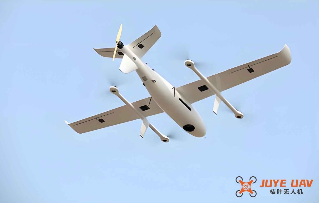
The ducted VTOL fixed-wing drone is a hybrid aircraft that integrates the vertical take-off, landing, and hovering capabilities of a helicopter with the high-speed, efficient cruise performance of a conventional fixed-wing drone. This combination makes it a highly promising platform for various military and civilian applications. The drone typically possesses three distinct flight states: the vertical take-off/landing and hovering state, the high-speed horizontal cruise state, and the critical transition state that links the first two. The transition state is the most complex, involving continuous changes in the configuration of propulsion units and flight attitude, which directly impacts the longitudinal stability of the fixed-wing drone. A key challenge is to accurately model the aerodynamic forces generated by the lift fan and the thrust duct, and to integrate these into a complete flight dynamics model to analyze longitudinal stability. In this paper, we present our work on developing such a model and applying it to a case study fixed-wing drone.
2. Aerodynamic Component Modeling
The accurate prediction of forces and moments from the propulsion system is crucial for the stability analysis of our fixed-wing drone. We developed separate models for the coaxial lift fan and the thrust duct, using the Blade Element Momentum Theory (BEMT) as the foundation, calibrated and refined with experimental data.
2.1 Lift Fan Aerodynamic Model
The coaxial contra-rotating lift fan is the primary vertical lift generator. We used the BEMT to model its performance. The BEMT formulation for the upper rotor is given by the following equations.
The non-dimensional inflow velocity for the upper rotor, $\lambda_u$, is solved from the combination of momentum and blade element theories. The basic equation is:
$$ \lambda(r, \lambda_{\infty}) = \sqrt{ \left( \frac{\sigma_u C_{l_\alpha}}{16F} – \frac{\lambda_\infty}{2} \right)^2 + \frac{\sigma_u C_{l_\alpha}}{8F} \theta_u r } – \left( \frac{\sigma_u C_{l_\alpha}}{16F} – \frac{\lambda_\infty}{2} \right) $$
where:
* $\sigma_u$ is the solidity of the upper rotor.
* $C_{l_\alpha}$ is the lift curve slope of the blade airfoil.
* $F$ is the Prandtl tip-loss factor.
* $\lambda_\infty$ is the non-dimensional free-stream velocity.
* $\theta_u$ is the blade pitch angle.
* $r$ is the non-dimensional radial position.
For the lower rotor, which operates partially in the wake of the upper rotor, the inflow velocity $\lambda_l$ is modified:
$$ \lambda_l(r) = \sqrt{ \left( \frac{\sigma_l C_{l_\alpha}}{16F} – \frac{\lambda_\infty + \lambda_u / a^2}{2} \right)^2 + \frac{\sigma_l C_{l_\alpha}}{8F} \theta_l r } – \left( \frac{\sigma_l C_{l_\alpha}}{16F} – \frac{\lambda_\infty + \lambda_u / a^2}{2} \right) $$
where $a$ is the wake contraction ratio ($a=0.707$ in the ideal case).
The thrust coefficient for the upper and lower rotors can be expressed as:
$$ C_{T_u} = \frac{1}{2} \int_0^1 \sigma_u C_{l_\alpha} (\theta_u r^2 – \lambda_u r) dr $$
$$ C_{T_l} = \frac{1}{2} \int_0^1 \sigma_l C_{l_\alpha} (\theta_l r^2 – \lambda_l r) dr $$
The total thrust of the co-axial system is $T = \rho A (\Omega R)^2 (C_{T_u} + C_{T_l})$.
To account for the effect of the duct, especially its lip, we introduced a correction factor $\eta$ to the inflow velocity of the upper rotor. This factor was identified from experimental data. Furthermore, we adopted a characteristic cross-section approach, using the aerodynamic data at $r/R = 0.6$ to represent the overall performance.
| Parameter | Description | Value/Model |
|---|---|---|
| $\eta$ | Duct lip correction factor for inflow | $\eta = f(V_\infty)$, determined from experiment |
| $r_c$ | Characteristic radial position | $r/R = 0.6$ |
| $C_{T_{fan}}$ | Total fan thrust coefficient | $C_{T_u} + C_{T_l}$ |
2.2 Thrust Duct Aerodynamic Model
The aft thrust duct provides forward propulsion during forward flight and can be vectored to provide vertical thrust during take-off and landing. The BEMT model for the thrust duct is similar, but without a tip-loss factor, and its lower surface is a stator.
The non-dimensional inflow velocity for the thrust duct’s upper rotor is:
$$ \lambda_{duct}^u = \sqrt{ \left( \frac{\sigma_u C_{l_\alpha}}{16} – \frac{\lambda_\infty}{2} \right)^2 + \frac{\sigma_u C_{l_\alpha}}{8} \theta_u r } – \left( \frac{\sigma_u C_{l_\alpha}}{16} – \frac{\lambda_\infty}{2} \right) \cdot \eta $$
The total thrust coefficient for the duct is then $C_{T}^{duct} = C_{T_u}$.
| Parameter | Description | Model Implementation |
|---|---|---|
| $\lambda_{duct}^u$ | Inflow velocity for duct upper rotor | BEMT with correction factor $\eta$ |
| $F$ | Prandtl tip-loss factor | Neglected (high blade count) |
| $V_{\infty}^{duct}$ | Free-stream velocity relative to duct | $V_{\infty} = -(V_z + qL_{ductG})\sin\theta_d + V_x\cos\theta_d$ |
3. Flight Dynamics Modeling of the Fixed-Wing Drone
The complete flight dynamics of the fixed-wing drone were modeled using the standard six-degree-of-freedom rigid-body equations. For the longitudinal stability analysis, we derived the linearized small-perturbation equations about a trim condition. The longitudinal state vector is defined as $X = [\Delta u, \Delta w, \Delta q, \Delta \theta]^T$.
The matrix form of the linearized equations is $A \dot{X} = B X$, where $A$ and $B$ contain the stability derivatives. The matrix $B$ is given by:
$$ B = \begin{bmatrix} \frac{\partial F_x}{\partial u} & \frac{\partial F_x}{\partial w} & \frac{\partial F_x}{\partial q} – m w^* & -mg \cos\theta^* \\ \frac{\partial F_z}{\partial u} & \frac{\partial F_z}{\partial w} & \frac{\partial F_z}{\partial q} + m u^* & mg \sin\theta^* \\ \frac{\partial M_y}{\partial u} & \frac{\partial M_y}{\partial w} & \frac{\partial M_y}{\partial q} & 0 \\ 0 & 0 & 1 & 0 \end{bmatrix} $$
The total aerodynamic forces and moments are a sum of contributions from the lift fan, the thrust duct, and the entire airframe (wing and body). The stability derivatives (e.g., $\partial F_x / \partial u$) are therefore also a sum of contributions from each component: $ \frac{\partial F_x}{\partial u} = \frac{\partial F_{x,fan}}{\partial u} + \frac{\partial F_{x,duct}}{\partial u} + \frac{\partial F_{x,wing}}{\partial u} $. The deflection of the thrust duct also changes the vehicle’s moment of inertia $I_y = f(\theta_{duct})$, which was accounted for in our model.
4. Case Study: Longitudinal Stability Analysis
We applied our model to a case study fixed-wing drone with a mass of 9.2 kg, a forward lift fan diameter of 460 mm, and a rear thrust duct diameter of 70 mm. We solved for the trim conditions and then analyzed the longitudinal stability for both hovering and transition flight.
4.1 Trim Condition and Balance Equations
**Hovering Trim**: In the hovering state, the forces must balance. The equilibrium equations in the body-fixed frame are:
$$ T_{duct}\cos\theta_{duct} – mg\sin\theta = 0 $$
$$ T_{fan} + T_{duct}\sin\theta_{duct} – mg\cos\theta = 0 $$
$$ T_{fan} l_{fan} – T_{duct} l_{duct}\sin\theta_{duct} = 0 $$
Solving these equations yields the required thrust values and duct deflection angle for a given pitch attitude $\theta$.
| Parameter | Symbol | Value | Unit |
|---|---|---|---|
| Lift Fan Thrust | $T_{fan}$ | 88.2 | N |
| Thrust Duct Thrust | $T_{duct}$ | 12.6 | N |
| Duct Deflection Angle | $\theta_{duct}$ | 90.0 | deg |
**Transition Trim**: During transition, the aerodynamic forces from the airframe ($L, D, M$) are significant. The equilibrium equations become:
$$ T_{duct}\cos\theta_{duct} + L_{wing}\sin\theta – mg\sin\theta – D_{wing}\cos\theta = 0 $$
$$ T_{fan} + T_{duct}\sin\theta_{duct} + L_{wing}\cos\theta + D_{wing}\sin\theta – mg\cos\theta = 0 $$
$$ M_{wing} + T_{fan} l_{fan} – T_{duct} l_{duct}\sin\theta_{duct} = 0 $$
4.2 Stability Results
The longitudinal stability was assessed by calculating the eigenvalues of the system matrix $A_s = A^{-1}B$ at various flight conditions.
**Hovering Stability**: From our analysis, the hovering state of the fixed-wing drone is longitudinally unstable for most pitch attitudes. The root locus for varying pitch angles ($-5^\circ$ to $10^\circ$) is shown below.
$$ \text{Eigenvalues: } \lambda_1, \lambda_2, \lambda_3, \lambda_4 $$
At a pitch angle of $0^\circ$, the system exhibits two zero roots and two negative real roots, indicating neutral stability and a monotonic convergence mode. For other pitch angles, the presence of roots with positive real parts (either a positive real root or a complex conjugate pair with a positive real part) leads to a divergent motion. This confirms that active control is required for stable hovering.
**Transition Stability**: Our analysis of transition flight is presented in two velocity ranges.
For low forward speeds (1-4 m/s), the fixed-wing drone remains longitudinally unstable. The eigenvalues show a mix of stable and unstable modes. This is shown in the following table.
| Eigenvalue Type | Number of Roots | Stability Implication |
|---|---|---|
| Conjugate complex pair (Re > 0) | 1 pair | Oscillatory divergence |
| Positive real | 1 | Monotonic divergence |
| Negative real | 1 | Monotonic convergence |
At forward speeds greater than 5 m/s, the longitudinal dynamics become stable. The eigenvalues consist of a stable conjugate complex pair (long-period phugoid mode) and two stable real roots (subsidence modes). This indicates that the fixed-wing drone’s inherent aerodynamic stability, derived from its wing and tail surfaces, begins to dominate.
| Eigenvalue Type | Number of Roots | Mode Description |
|---|---|---|
| Conjugate complex pair (both Re < 0) | 1 pair | Stable long-period (phugoid) mode |
| Stable real roots | 2 | Overdamped modes |
Our experimental hover testing corroborated these findings. The measured oscillation period of a pitch disturbance was approximately 7 seconds, which matches the calculated period of the oscillatory mode in the hover analysis, validating the accuracy of our model.
5. Conclusion
In this work, we successfully developed a comprehensive model to study the longitudinal stability of a ducted vertical take-off and landing fixed-wing drone. Our key findings and contributions are:
1. **Accurate Propulsion Models**: We developed aerodynamic models for a coaxial ducted lift fan and a thrust duct based on BEMT. By incorporating a correction factor derived from experimental data and using a characteristic cross-section approach, our models predicted the thrust with an error of less than 5%.
2. **Complete Flight Dynamics Model**: An integrated flight dynamics model was established using the six-degree-of-freedom equations, which effectively accounts for the deflection of the thrust duct and its impact on vehicle inertia. This model is capable of describing the longitudinal motion of the fixed-wing drone.
3. **Stability Characteristics**: Our analysis revealed the following:
* The hovering state of the fixed-wing drone is longitudinally unstable, requiring active control for stabilization.
* During the transition, the fixed-wing drone is unstable at low airspeeds (1-4 m/s).
* At airspeeds above 5 m/s, the fixed-wing drone’s inherent aerodynamic stability stabilizes the longitudinal motion.
The methodology and findings presented here provide a solid foundation for future work on the control system design and broader flight dynamics of this class of ducted VTOL fixed-wing drones. Future research will focus on lateral-directional stability and the handling qualities of the full flight envelope.