
Our study investigated the potential of combining spectral and textural information extracted from fixed-wing drone multispectral imagery to monitor key rice growth indicators, namely leaf area index (LAI), aboveground biomass (AGB), and plant nitrogen content (PNC). We conducted two years of field experiments involving multiple rice varieties, sowing dates, transplanting methods, and nitrogen application rates. During critical growth stages, we acquired canopy multispectral images using a fixed-wing drone equipped with a Sequoia camera and simultaneously collected destructive samples to measure LAI, AGB, and PNC. Simple linear regression (SLR), partial least squares regression (PLSR), and artificial neural network (ANN) were employed to build monitoring models. Our results demonstrate that the fusion of vegetation indices (VIs) and texture indices (TIs) as inputs into ANN significantly outperformed models using only spectral or texture features alone. The optimal ANN model achieved validation R² values of 0.86 for LAI, 0.92 for AGB, and 0.86 for PNC, with corresponding RMSE reductions compared to SLR models. This research highlights the effectiveness of fixed-wing drone multispectral data combined with machine learning for accurate, non-destructive assessment of rice growth status, providing a practical approach for large-scale crop management.
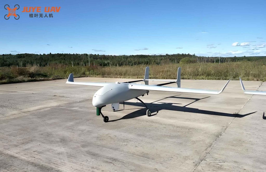
The rapid and accurate monitoring of crop growth status is essential for precision agriculture. Among various remote sensing platforms, the fixed-wing drone offers distinct advantages over multi-rotor drones, including longer flight endurance and greater coverage area, making it particularly suitable for large-scale agricultural surveys. In this study, we employed a fixed-wing drone (eBee-SQ) carrying a Parrot Sequoia multispectral camera, which captures images in green, red, red-edge, and near-infrared bands. With a flight height of 80 m, the system achieved a ground resolution of 8 cm and covered approximately 90 hectares per flight. The fixed-wing drone platform thus provided an efficient means to collect high-resolution multispectral data over extensive rice fields.
Materials and Methods
Experimental Design and Data Acquisition
We conducted field experiments over two consecutive growing seasons using a randomized complete block design with three replicates. Treatments included three rice varieties (two in the first year, three in the second), four nitrogen levels (0, 135, 270, and 405 kg·ha⁻¹), and two transplanting methods (tray seedling and blanket seedling). The plots were managed under standard practices for pest and water control. At key growth stages (tillering, jointing, booting, heading), we collected three representative hills per plot to measure LAI (via leaf area meter), AGB (after oven-drying at 80°C to constant weight), and PNC (using the Kjeldahl method). Simultaneously, the fixed-wing drone flew over the experiment site between 10:00 and 14:00 under clear skies. Images were processed using Pix4Dmapper to generate orthomosaics and single-band reflectance maps. Radiometric calibration was performed using a standard reflectance panel captured before each flight.
Image Processing and Feature Extraction
We extracted spectral information by calculating the mean reflectance of each plot from the four bands. Six commonly used vegetation indices (VIs) were computed (Table 1). For texture analysis, we applied the gray-level co-occurrence matrix (GLCM) with a 3×3 window, step size of 1, and averaged over four directions (0°, 45°, 90°, 135°). Eight texture features were extracted per band: mean (Mea), variance (Var), homogeneity (Hom), contrast (Con), dissimilarity (Dis), entropy (Ent), second moment (Sec), and correlation (Cor). To enhance texture information, we constructed normalized difference texture indices (NDTI), ratio texture indices (RTI), and difference texture indices (DTI) by pairing texture features from different bands (Table 2).
| Vegetation Index | Abbreviation | Formula |
|---|---|---|
| Normalized Difference Vegetation Index | NDVI | $$ \frac{NIR – R}{NIR + R} $$ |
| Normalized Difference Red-Edge Index | NDRE | $$ \frac{NIR – RE}{NIR + RE} $$ |
| Ratio Vegetation Index | RVI | $$ \frac{NIR}{R} $$ |
| Difference Vegetation Index | DVI | $$ NIR – R $$ |
| Red-Edge Soil-Adjusted Vegetation Index | RESAVI | $$ 1.5 \times \frac{NIR – RE}{NIR + RE + 0.5} $$ |
| Red-Edge Chlorophyll Index | CIRE | $$ \frac{NIR}{RE} – 1 $$ |
| Texture Index | Abbreviation | Formula |
|---|---|---|
| Normalized Difference Texture Index | NDTI | $$ \frac{T_1 – T_2}{T_1 + T_2} $$ |
| Ratio Texture Index | RTI | $$ \frac{T_1}{T_2} $$ |
| Difference Texture Index | DTI | $$ T_1 – T_2 $$ |
Note: T₁ and T₂ represent texture feature values (e.g., Mea, Var) extracted from two different bands.
Model Development and Evaluation
We employed three modeling approaches: SLR, PLSR, and ANN. For SLR, we regressed LAI, AGB, and PNC against individual VIs or selected TIs. PLSR was implemented using the pls package in R, with the optimal number of principal components determined by leave-one-out cross-validation. The ANN model was a multi-layer perceptron with one hidden layer (3–30 neurons), hyperbolic tangent activation, and identity output. Input variables included either VIs alone or VIs plus the six best-performing TIs. Models were calibrated using 70% of the data (stratified across years and treatments) and validated with the remaining 30%. Performance was assessed via the coefficient of determination (R²) and root mean square error (RMSE). Variable importance in projection (VIP) scores were computed for PLSR and ANN to evaluate the contribution of each input variable.
Results
Variability of Rice Growth Indicators
The dataset covered a wide range of growth conditions, as shown in Table 3. LAI ranged from 0.40 to 9.07, AGB from 0.66 to 21.94 t·ha⁻¹, and PNC from 0.56% to 3.88%. Coefficients of variation exceeded 34% for all three parameters, indicating sufficient variability for robust model development.
| Indicator | Min | Max | Mean | SD | CV (%) |
|---|---|---|---|---|---|
| LAI | 0.40 | 9.07 | 3.69 | 1.94 | 52.57 |
| AGB (t·ha⁻¹) | 0.66 | 21.94 | 7.87 | 5.57 | 70.78 |
| PNC (%) | 0.56 | 3.88 | 1.93 | 0.66 | 34.20 |
Performance of Vegetation Indices Alone
Simple linear regression using individual VIs revealed strong correlations with LAI and AGB, but weak correlations with PNC (Table 4). The best VIs for LAI and AGB were CIRE (R²=0.80) and NDRE (R²=0.76), respectively. For PNC, the maximum R² was only 0.13 (RESAVI and NDRE). Validation of the SLR models using independent data confirmed these trends: LAI (R²=0.75, RMSE=0.99), AGB (R²=0.72, RMSE=3.12), and PNC (R²=0.26, RMSE=0.55). These results indicate that spectral information alone is insufficient for PNC estimation, and that texture features may provide complementary information.
| VI | LAI | AGB | PNC |
|---|---|---|---|
| NDVI | 0.49 | 0.37 | 0.08 |
| NDRE | 0.78 | 0.76 | 0.13 |
| RVI | 0.49 | 0.34 | 0.06 |
| DVI | 0.61 | 0.61 | 0.11 |
| CIRE | 0.80 | 0.75 | 0.12 |
| RESAVI | 0.77 | 0.74 | 0.13 |
Performance of Texture Features and Texture Indices
Single-band texture features (e.g., Mea, Var) showed weaker correlations with LAI and AGB compared to VIs. The highest R² for LAI was 0.48 (Mea from the near-infrared band), and for AGB it was 0.43 (Mea from the green band). PNC correlations with single texture features were negligible (max R²=0.09). However, after constructing texture indices by pairing features from different bands, the correlations improved (Table 5). The best texture index for LAI was NDTI(Mea₅₅₀, Mea₇₉₀) with R²=0.59; for AGB, the same index gave R²=0.48; for PNC, DTI(Sec₇₃₅, Ent₆₆₀) achieved R²=0.26. Notably, the texture indices for PNC outperformed any single VI, suggesting that texture captures nitrogen-related structural variation that spectral reflectance alone misses.
| Indicator | Top TI | R² |
|---|---|---|
| LAI | NDTI(Mea₅₅₀, Mea₇₉₀) | 0.59 |
| AGB | NDTI(Mea₅₅₀, Mea₇₉₀) | 0.48 |
| PNC | DTI(Sec₇₃₅, Ent₆₆₀) | 0.26 |
PLSR Models Using VIs and VIs + TIs
When we built PLSR models using only the six VIs, the validation performance improved slightly over the best SLR models (Table 6). Adding the six selected TIs further enhanced accuracy, especially for AGB and PNC. For AGB, the validation R² increased from 0.73 (VIs alone) to 0.81 (VIs+TIs), while RMSE dropped from 3.04 to 2.52 t·ha⁻¹. For PNC, R² improved from 0.27 to 0.36, and RMSE decreased from 0.53% to 0.48%. The LAI model showed marginal improvement (R² from 0.76 to 0.77). VIP analysis indicated that for LAI and AGB, the most important inputs were CIRE, NDRE, and RESAVI, while for PNC, texture indices such as DTI(Cor₅₅₀, Sec₆₆₀) and RTI(Var₆₆₀, Con₆₆₀) had higher VIP values than most VIs.
| Input set | LAI R² | LAI RMSE | AGB R² | AGB RMSE (t·ha⁻¹) | PNC R² | PNC RMSE (%) |
|---|---|---|---|---|---|---|
| VIs only | 0.76 | 0.97 | 0.73 | 3.04 | 0.27 | 0.53 |
| VIs + TIs | 0.77 | 0.96 | 0.81 | 2.52 | 0.36 | 0.48 |
ANN Models Using VIs and VIs + TIs
ANN models consistently outperformed both SLR and PLSR. When only VIs were used, the best ANN (with optimal hidden neurons) achieved validation R² of 0.85, 0.88, and 0.53 for LAI, AGB, and PNC, respectively (Table 7). Adding the six TIs further boosted performance: LAI R² reached 0.86, AGB R² 0.92, and PNC R² 0.86. The RMSE for PNC dropped dramatically from 0.46% (VIs alone) to 0.25% (VIs+TIs), representing a 46% reduction. The ANN architecture for the best combined model used 25 neurons for LAI, 29 for AGB, and 30 for PNC. VIP scores from the ANN revealed that the texture indices contributed significantly to PNC estimation, while VIs remained dominant for LAI and AGB.
| Input set | LAI R² | LAI RMSE | AGB R² | AGB RMSE (t·ha⁻¹) | PNC R² | PNC RMSE (%) |
|---|---|---|---|---|---|---|
| VIs only | 0.85 | 0.74 | 0.88 | 1.86 | 0.53 | 0.46 |
| VIs + TIs | 0.86 | 0.72 | 0.92 | 1.56 | 0.86 | 0.25 |
Overall Comparison of Modeling Approaches
Table 8 summarizes the validation performance across all methods and input combinations. Clearly, the ANN model with combined VIs and TIs yielded the highest accuracy for all three growth indicators. The improvements were most pronounced for PNC, where the R² increased from 0.26 (SLR with best VI) to 0.86 (ANN with VIs+TIs). For LAI and AGB, the ANN also delivered substantial gains. The fixed-wing drone multispectral imagery, when processed with advanced machine learning, thus enables reliable non-destructive monitoring of rice growth parameters over large areas.
| Model & Input | LAI R² | LAI RMSE | AGB R² | AGB RMSE (t·ha⁻¹) | PNC R² | PNC RMSE (%) |
|---|---|---|---|---|---|---|
| SLR (best VI) | 0.75 | 0.99 | 0.72 | 3.12 | 0.26 | 0.55 |
| PLSR (VIs+TIs) | 0.77 | 0.96 | 0.81 | 2.52 | 0.36 | 0.48 |
| ANN (VIs) | 0.85 | 0.74 | 0.88 | 1.86 | 0.53 | 0.46 |
| ANN (VIs+TIs) | 0.86 | 0.72 | 0.92 | 1.56 | 0.86 | 0.25 |
Discussion
Our findings demonstrate that the fixed-wing drone platform offers significant operational advantages for agricultural remote sensing. With a single flight covering up to 90 ha, it is well suited for regional-scale crop monitoring. The combination of spectral and textural features proved crucial for improving estimation accuracy, especially for PNC, where spectral indices alone were inadequate. This aligns with previous studies that reported texture features can mitigate saturation effects in dense canopies and capture structural variations related to nitrogen status. The texture indices derived from green and near-infrared bands were particularly effective for LAI and AGB, likely because the green band is sensitive to pigment content and the near-infrared band responds to canopy structure and biomass. For PNC, texture indices involving the red-edge band (e.g., entropy and second moment) performed best, as the red-edge region is known to be sensitive to chlorophyll and nitrogen concentration.
The superiority of ANN over PLSR and SLR can be attributed to its ability to model non-linear relationships among input variables. The fixed-wing drone imagery provides high-dimensional data (reflectance at four bands plus multiple texture features), and ANN can exploit complex interactions that linear or weakly non-linear methods cannot. The VIP analysis confirmed that different indicators benefited from different combinations: for LAI and AGB, VIs with red-edge bands (CIRE, NDRE) dominated, while for PNC, texture features contributed more. This suggests that a multi-feature fusion strategy is essential for comprehensive crop monitoring.
Despite the promising results, some limitations should be acknowledged. The impact of spatial resolution on texture extraction was not explored; different window sizes and flight altitudes could affect optimal texture selection. Additionally, our dataset came from only two years and two locations; further validation across diverse environments and years is needed to ensure model robustness. Future work could incorporate canopy height information (e.g., from structure-from-motion) or temporal series to improve predictions further. Nevertheless, our study provides strong evidence that fixed-wing drone multispectral imagery, when combined with advanced machine learning and texture features, can reliably estimate key rice growth indicators, offering a practical tool for precision agriculture.
Conclusion
This research successfully demonstrated the use of a fixed-wing drone equipped with a multispectral camera for non-destructive monitoring of rice LAI, AGB, and PNC. By fusing spectral vegetation indices with texture indices derived from GLCM, and applying an artificial neural network, we achieved high accuracy in estimating all three growth parameters. The final ANN model using combined VIs and TIs yielded validation R² values of 0.86, 0.92, and 0.86 for LAI, AGB, and PNC, respectively, with significantly reduced RMSE compared to simpler methods. The fixed-wing drone platform proved to be an efficient and scalable data acquisition system for large-scale crop monitoring. Our approach provides a reliable technical solution for real-time, field-level assessment of rice growth status, supporting precise nitrogen management and yield prediction.