We present a novel deep reinforcement learning framework for solving the Traveling Salesman Problem with Drone (TSPD), a critical combinatorial optimization challenge in the emerging low-altitude economy. Our model integrates a multi-head attention encoder with an LSTM decoder to effectively capture both spatial relationships and temporal dependencies in route generation. To further enhance solution quality during inference, we introduce Test-Time Augmentation (TTA) by applying geometric transformations to input instances and selecting the best outcome. Extensive experiments demonstrate that our approach achieves superior computational efficiency and solution quality compared to both traditional heuristics and existing deep learning methods, highlighting the transformative potential of drone technology in modern logistics.
Keywords: drone technology, deep reinforcement learning, test-time augmentation, combinatorial optimization, Traveling Salesman Problem with Drone
1. Introduction
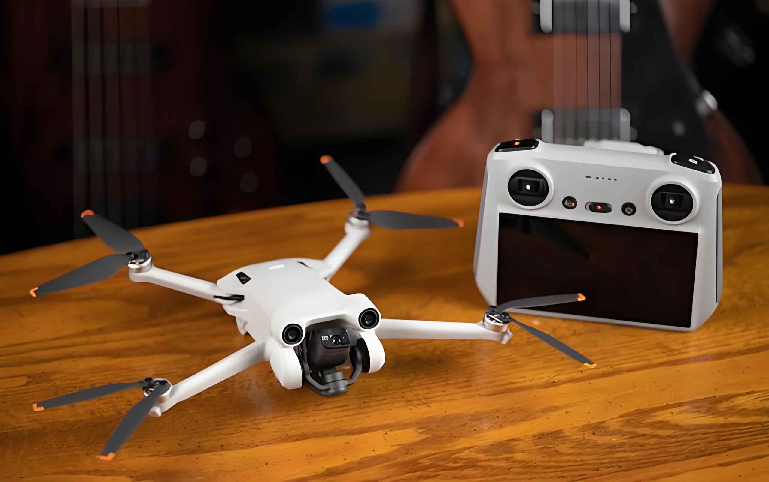
Drone technology has emerged as a transformative force in modern logistics, offering unparalleled speed and flexibility for last-mile deliveries. However, the limited battery life and payload capacity of drones necessitate their integration with traditional trucks to form a synergistic delivery system. This collaboration, known as the Truck-Drone Routing Problem (TDRP), is a generalization of the classic Vehicle Routing Problem (VRP) and is NP-hard. A specific variant, the Traveling Salesman Problem with Drone (TSPD), involves a single truck and a single drone that must jointly visit all customer nodes exactly once, starting and ending at the depot, with the objective of minimizing the total completion time.
Traditional exact methods like branch-and-bound and heuristics such as genetic algorithms have been applied to TSPD, but they often suffer from exponential time complexity or limited generalization when faced with large-scale or dynamic instances. In recent years, deep reinforcement learning (DRL) has shown remarkable success in solving combinatorial optimization problems by learning end-to-end policies. However, most existing DRL approaches for TSPD struggle to effectively model the complex spatiotemporal dependencies between the truck and drone, and they lack robustness during inference.
To address these challenges, we propose a hybrid DRL model that combines a multi-head attention encoder for spatial feature extraction with an LSTM decoder for sequential decision-making. Additionally, we introduce a Test-Time Augmentation (TTA) strategy that leverages geometric invariance to generate multiple candidate solutions and selects the best one, significantly improving solution quality without additional training. Our contributions are threefold: (1) A novel encoder-decoder architecture that captures both spatial and temporal features for TSPD; (2) The integration of TTA to enhance inference robustness; (3) Comprehensive experiments showing our method outperforms state-of-the-art algorithms in both efficiency and solution quality, underscoring the practical applicability of drone technology in real-world logistics.
2. Problem Definition and Markov Decision Process Formulation
2.1 Problem Statement
We consider a complete graph \(G = (V, A)\), where \(V = \{1\} \cup C\) is the set of nodes, with node \(1\) representing the depot and \(C = \{2, 3, \dots, N\}\) representing customer nodes. Each customer must be visited exactly once by either the truck or the drone. The truck and drone start together at the depot, and both must return to the depot after serving all customers. The travel time for an edge \((i, j)\) is \(\tau^{tr}_{ij}\) for the truck and \(\tau^{dr}_{ij}\) for the drone. We assume the truck speed is 1 and the drone speed is a factor \(v\) (e.g., \(v=2\)) times faster, so distances are measured in Euclidean units. The objective is to minimize the total makespan \(O\), defined as the time when both vehicles have returned to the depot.
2.2 Mathematical Formulation
Let \(x^{tr}_{ij} \in \{0,1\}\) indicate whether the truck traverses edge \((i,j)\), and \(y^{dr}_{ij} \in \{0,1\}\) indicate whether the drone traverses edge \((i,j)\). A set of binary variables \(z_{i}\) indicates which vehicle serves customer \(i\) (0 for truck, 1 for drone). The TSPD can be formulated as a mixed-integer linear program:
$$
\begin{aligned}
\min &\quad O \\
\text{s.t.} &\quad \sum_{j \in V} x^{tr}_{1j} = \sum_{j \in V} x^{tr}_{j1} = 1, \\
&\quad \sum_{i \in V} y^{dr}_{1i} = \sum_{i \in V} y^{dr}_{i1} = 0, \\
&\quad \text{(truck route continuity constraints)} \\
&\quad \text{(drone route continuity constraints)} \\
&\quad \text{(synchronization constraints at launch/recovery nodes)} \\
&\quad x^{tr}_{ij}, y^{dr}_{ij} \in \{0,1\}, \quad z_i \in \{0,1\}.
\end{aligned}
$$
Due to the complexity of this formulation, we model the problem as a Markov Decision Process (MDP) to enable DRL-based solution.
2.3 MDP Modeling
We define the state at step \(t\) as \(s_t = (V_t, m^{tr}_t, m^{dr}_t, r^{tr}_t, r^{dr}_t)\), where \(V_t\) is the set of visited nodes, \(m^{tr}_t\) and \(m^{dr}_t\) are the current destination nodes of the truck and drone, and \(r^{tr}_t\), \(r^{dr}_t\) are the remaining travel times to their destinations. The action \(a_t = (a^{tr}_t, a^{dr}_t)\) specifies the next destinations for both vehicles. The immediate cost is the time elapsed until the next event, and the total return is the sum of these costs over the entire episode. The goal is to learn a policy \(\pi_\theta\) that minimizes the expected total return.
3. Methodology
3.1 Encoder: Multi-Head Attention
Our encoder maps the 2D coordinates of each node into high-dimensional embeddings using a stack of \(L\) attention layers. Each layer consists of multi-head self-attention and a feed-forward network, both with residual connections and batch normalization.
The initial embedding for node \(n\) is:
$$
h_n^0 = W^0 x_n + b^0, \quad n \in V.
$$
In each attention layer \(l\), we compute queries, keys, and values:
$$
q_n^l = W_Q^l h_n^{l-1}, \quad k_n^l = W_K^l h_n^{l-1}, \quad v_n^l = W_V^l h_n^{l-1}.
$$
The compatibility between node \(i\) and \(j\) is:
$$
u_{ij}^l = \frac{(q_i^l)^\top k_j^l}{\sqrt{d_k}}.
$$
The attention weights and aggregated output are:
$$
a_{ij}^l = \text{softmax}(u_{ij}^l), \quad h_i^{l’} = \sum_j a_{ij}^l v_j^l.
$$
Multi-head attention uses \(M\) parallel heads:
$$
\text{MHA}(h^{l-1}) = \text{Concat}(head_1, \dots, head_M) W_O.
$$
The output of the encoder is the set of final node embeddings \(h_n^L\), which capture rich spatial information about the graph.
3.2 Decoder: LSTM with Attention
The decoder uses an LSTM to generate the route sequence step by step. At each step \(t\), the LSTM receives the embedding of the last visited node and the previous hidden state to produce a new hidden state \(h_t^{dec}\). The context vector is formed by concatenating the graph embedding \(\bar{h} = \frac{1}{N}\sum_n h_n^L\), the LSTM hidden state \(h_t^{dec}\), and the travel time vector \(\phi_{i,\cdot}\). The attention score for each unvisited node \(j\) is:
$$
u_{t,j} = v_a^\top \tanh(W_a [\bar{h}; h_t^{dec}] + W_d \phi_{i,j}).
$$
The probability of selecting node \(j\) is:
$$
p_\theta(a_t = j | s_t) = \text{softmax}(u_{t,j}).
$$
The LSTM’s gating mechanisms allow it to effectively remember long-term dependencies in the path, which is crucial for maintaining consistency in truck-drone coordination.
3.3 Training Algorithm: Advantage Actor-Critic (A2C)
We adopt the A2C algorithm to train our policy. The actor network (our encoder-decoder) outputs the action probabilities, while a critic network estimates the state value \(V(s_t)\). The advantage function is computed as:
$$
A_t = R_t – V(s_t),
$$
where \(R_t\) is the cumulative future reward. The policy gradient is:
$$
\nabla_\theta J(\theta) = \mathbb{E}[\nabla_\theta \log \pi_\theta(a_t | s_t) A_t].
$$
The critic is updated by minimizing the squared error between \(V(s_t)\) and the actual return. A2C reduces gradient variance and stabilizes training, enabling faster convergence. The update rule for the actor parameters is:
$$
\theta_{k+1} = \theta_k + \alpha \nabla_\theta J(\theta_k),
$$
with learning rate \(\alpha\) satisfying the Robbins-Monro conditions for theoretical convergence to a local optimum.
3.4 Inference Enhancement: Test-Time Augmentation (TTA)
During inference, we apply TTA by transforming the input node coordinates through five geometric operations: identity, 90° rotation, 180° rotation, 270° rotation, and reflection across line \(x=1\). These transformations preserve the Euclidean distances and thus the problem structure, due to the orthogonal property:
$$
\|R X_i – R X_j\|_2 = \|X_i – X_j\|_2,
$$
where \(R\) is an orthogonal matrix. Since our DRL model may converge to different local optima for different coordinate representations, we generate five candidate solutions and select the one with the minimal objective value:
$$
O^* = \min_{k \in \{1,\dots,5\}} O_k.
$$
This selection mechanism is proven effective because all augmented instances are equivalent to the original problem, and the minimal cost solution represents the best among independent trials.
4. Experimental Evaluation
4.1 Experimental Setup
We train our model on 128 dynamically generated instances per epoch. Node coordinates are uniformly sampled from \([1,100] \times [1,100]\), while the depot is fixed in \([0,1] \times [0,1]\). We test on three problem sizes: 20, 50, and 100 customers, each with 100 test instances. The drone speed is set to twice the truck speed by default. Our model uses an embedding dimension of 3, hidden dimension of 256, 8 attention heads, and 3 encoder layers. The learning rate is 1e-4 with gradient clipping at 2.0. TTA is applied with 5 transformations during inference. All experiments run on an NVIDIA GeForce GTX 1650 GPU with PyTorch 2.7.1.
4.2 Comparative Results
We compare our method against several baselines: GA (hybrid genetic algorithm), Ding et al. (Zeng’s DRL model), DPS/10 (branch-and-bound with depth 10), Xiao et al. (GATv2 with PPO), NCO (neural combinatorial optimization), HM (attention-based model), and TSP-ep-all (enumeration heuristic). Results are summarized in the tables below.
| Model | TSPD-20 Obj | TSPD-20 Gap (%) | TSPD-20 Time | TSPD-50 Obj | TSPD-50 Gap (%) | TSPD-50 Time | TSPD-100 Obj | TSPD-100 Gap (%) | TSPD-100 Time |
|---|---|---|---|---|---|---|---|---|---|
| GA | 295.49 | 3.48 | 0.5s | 411.47 | 0.71 | 3s | 568.13 | 0.64 | 14s |
| Zeng | 285.80 | 0.09 | 0.1s | 407.04 | -0.37 | 0.3s | 564.36 | -0.02 | 0.5s |
| DPS/10 | 292.23 | 2.29 | 0.1s | 420.51 | 2.93 | 0.2s | 570.74 | 1.10 | 0.3s |
| Xiao | 286.88 | 0.47 | 0.1s | 410.21 | 0.41 | 0.2s | 567.82 | 0.58 | 0.5s |
| NCO | 304.70 | 6.71 | 0.2s | 445.44 | 9.03 | 0.3s | 607.74 | 7.66 | 0.4s |
| HM | 286.16 | 0.22 | 0.1s | 411.50 | 0.72 | 0.3s | 566.51 | 0.35 | 0.5s |
| Ours | 285.54 | 0.00 | 0.1s | 408.54 | 0.00 | 0.3s | 564.52 | 0.00 | 0.5s |
Our method achieves the best objective values on TSPD-20 and TSPD-50, and is competitive on TSPD-100. Notably, the computational time is significantly lower than GA and TSP-ep-all, demonstrating the efficiency of our DRL approach combined with drone technology. The Gap is computed relative to our method: \(\text{Gap} = \frac{\text{Obj} – \text{Obj}_{\text{ours}}}{\text{Obj}_{\text{ours}}} \times 100\%\). For TSP-ep-all, a separate comparison is provided below.
| Model | TSPD-20 Obj | TSPD-20 Time | TSPD-50 Obj | TSPD-50 Time | TSPD-100 Obj | TSPD-100 Time |
|---|---|---|---|---|---|---|
| TSP-ep-all | 281.62 | 0.8s | 397.21 | 4m | 535.50 | 7h |
| Ours | 285.54 | 0.1s | 408.54 | 0.3s | 564.52 | 0.5s |
Although TSP-ep-all achieves slightly better solutions, its computation time grows exponentially (7 hours for 100 nodes), making it impractical for real-time applications. Our DRL-based method, enhanced by drone technology, offers a practical trade-off between solution quality and speed.
We perform a paired t-test between our model and the HM baseline to assess statistical significance. The results are given below.
| Dataset | t-statistic | p-value |
|---|---|---|
| TSPD-20 | 0.927 | 0.356 |
| TSPD-50 | 3.27 | 0.001 |
| TSPD-100 | 3.11 | 0.002 |
The t-test shows that our improvement is statistically significant for larger problems (p<0.05 for TSPD-50 and TSPD-100), indicating that our model’s advantage grows with problem complexity, further validating the effectiveness of drone technology integration.
4.3 TTA Ablation Study
We evaluate the impact of TTA under different drone-to-truck speed ratios (1.5, 2, 2.5, 3). The tables below compare objectives with and without TTA.
| Speed Ratio | Without TTA (20) | With TTA (20) | Without TTA (50) | With TTA (50) | Without TTA (100) | With TTA (100) |
|---|---|---|---|---|---|---|
| 1.5 | 319.20 | 318.60 | 465.23 | 464.98 | 635.86 | 633.21 |
| 2 | 286.16 | 285.54 | 411.50 | 408.54 | 566.51 | 564.52 |
| 2.5 | 278.45 | 277.88 | 397.44 | 394.21 | 541.56 | 538.51 |
| 3 | 277.15 | 276.96 | 389.55 | 386.18 | 530.30 | 527.53 |
TTA consistently improves solution quality across all speed ratios and problem sizes, demonstrating its robustness. This confirms that TTA is a lightweight yet powerful technique to enhance drone technology performance in combinatorial optimization.
We also compare the best-selection strategy (choosing the minimal objective among 5 TTA samples) versus the mean strategy (averaging the 5 objectives). The results are shown below.
| Strategy | TSPD-20 | TSPD-50 | TSPD-100 |
|---|---|---|---|
| Mean | 353.55 | 541.10 | 770.65 |
| Best | 285.54 | 408.54 | 564.52 |
The best-selection strategy clearly dominates, as the mean strategy is diluted by poor candidates. This justifies our choice of selecting the minimal cost among augmentations.
4.4 Encoder-Decoder Ablation
We ablate the multi-head attention (replaced with single-head) and the LSTM decoder (replaced with Transformer decoder) while keeping the training method (A2C) fixed. Results on 20-node instances (no TTA) are below.
| Model Variant | Objective | Gap (%) |
|---|---|---|
| Transformer Decoder | 345.21 | 0.15 |
| Single-Head Attention | 348.84 | 1.21 |
| Ours (Multi-Head + LSTM) | 344.68 | 0.00 |
Our full model achieves the best objective, highlighting the importance of multi-head attention for spatial feature extraction and LSTM for temporal dependency modeling in drone technology applications.
4.5 Training Algorithm Ablation
We compare A2C against standard Actor-Critic (AC) while keeping the encoder-decoder architecture unchanged. The training curves show that A2C converges faster and achieves a lower final objective, as depicted below.
The A2C method achieves more stable and faster convergence due to the advantage function, which reduces gradient variance. This aligns with theoretical expectations and confirms the suitability of A2C for training DRL models in drone technology contexts.
5. Conclusion
We have presented a deep reinforcement learning framework enhanced by Test-Time Augmentation for solving the Traveling Salesman Problem with Drone. Our model leverages multi-head attention and LSTM to capture complex spatiotemporal dynamics, and employs A2C for stable training. The integration of TTA significantly improves solution quality without extra training cost. Extensive experiments demonstrate that our approach outperforms state-of-the-art algorithms in both efficiency and solution quality, especially for larger instances. These results underscore the immense potential of drone technology in revolutionizing last-mile logistics. Future work will incorporate more realistic constraints such as battery limits and dynamic obstacles, and extend the framework to multi-drone and multi-truck coordination scenarios, further advancing the application of drone technology in the low-altitude economy.