
In recent years, China UAV technology has advanced rapidly, enabling applications in logistics, agriculture, surveillance, and disaster response. Autonomous navigation in complex, dynamic environments remains a critical challenge for China UAV fleets. We propose a hierarchical reinforcement learning (HRL) framework that separates global planning and local control to improve convergence speed, collision avoidance, and path optimality. Our system consists of a high-level planner that generates temporary waypoints using a static global path and real-time point cloud data, and a low-level controller that tracks these waypoints at a higher frequency. Both modules are trained using the Soft Actor-Critic (SAC) algorithm with maximum entropy, ensuring robust exploration. Experimental results in simulated urban environments demonstrate that our approach achieves a 97.7% navigation success rate and 91.8% obstacle avoidance rate, outperforming single-layer and baseline HRL methods. This work contributes to the development of intelligent China UAV navigation systems capable of safe and efficient autonomous flight.
1. Introduction
The growing demand for China UAV applications in smart cities, emergency response, and aerial delivery has highlighted the need for reliable autonomous navigation. Traditional path planning methods, such as A*, RRT*, and trajectory optimization, often rely on precise environmental models and struggle with dynamic obstacles. Recent advances in deep reinforcement learning (DRL) offer end-to-end learning from sensor inputs to control commands, but they suffer from sparse rewards and high-dimensional state spaces. Hierarchical reinforcement learning (HRL) addresses these issues by decomposing the task into a high-level planner that sets subgoals and a low-level controller that executes actions. In the context of China UAV navigation, HRL can leverage global map information while adapting to local disturbances.
We introduce a novel HRL framework tailored for China UAVs. The high-level planner operates at 10 Hz and generates temporary target points relative to the UAV’s body frame, based on a precomputed global path and a 40×64 polar coordinate point cloud feature map. The low-level controller runs at 150 Hz and uses SAC to track these targets with high precision. The two layers are trained sequentially: first the low-level controller, then the high-level planner with the low-level controller fixed. This architecture implicitly embeds dynamic constraints into the high-level planner, improving overall robustness. Our contributions include a polar representation of LiDAR data for efficient obstacle encoding, a frequency-matching mechanism for asynchronous cooperation, and a maximum-entropy training strategy that accelerates convergence. Extensive simulations validate the effectiveness of the proposed system for China UAV navigation in cluttered environments.
2. Problem Formulation and System Modeling
We consider a quadrotor China UAV operating in a three-dimensional urban environment. The UAV is equipped with a laser radar that provides point cloud measurements up to a 10 m range. The task is to navigate from a given start point to a goal location while avoiding both static and dynamic obstacles. We model the problem as a Markov Decision Process (MDP) defined by the tuple (S, A, P, R, γ).
State Space: For the low-level controller, the state includes Euler angles (φ, θ, ψ), angular rates (p, q, r), position (x, y, z), linear velocities (vx, vy, vz), desired velocity, previous action, and the target point in body frame. For the high-level planner, the state consists of the UAV’s position in global coordinates, the expected guide point from the global path, and a polar coordinate point cloud feature map.
Action Space: The low-level controller outputs angular rates (p, q, r) and total thrust F. The high-level planner outputs a temporary target point [px, py, pz] in the UAV’s body frame.
Quadrotor Dynamics: Under standard assumptions (rigid body, symmetric mass distribution, negligible air resistance), we use the Newton-Euler equations. The rotational dynamics in the body frame are:
$$ \begin{aligned} \ddot{\phi} &= \frac{(I_{yy} – I_{zz}) q r + \tau_x – J_{RP} q \Omega}{I_{xx}} \\ \ddot{\theta} &= \frac{(I_{zz} – I_{xx}) p r + \tau_y + J_{RP} p \Omega}{I_{yy}} \\ \ddot{\psi} &= \frac{(I_{xx} – I_{yy}) p q + \tau_z}{I_{zz}} \end{aligned} $$
where Ω = -ω1 – ω2 + ω3 + ω4 is the rotor speed difference, and JRP is the total moment of inertia of rotors and propellers. The translational dynamics are:
$$ \begin{aligned} \ddot{x} &= (\cos\phi\sin\theta\cos\psi + \sin\phi\sin\psi) F / m \\ \ddot{y} &= (\cos\phi\sin\theta\sin\psi – \sin\phi\cos\psi) F / m \\ \ddot{z} &= g – (\cos\phi\cos\theta) F / m \end{aligned} $$
The control allocation matrix relates total thrust and moments to individual rotor speeds:
$$ \begin{bmatrix} F \\ \tau_1 \\ \tau_2 \\ \tau_3 \end{bmatrix} = l \begin{bmatrix} 1 & 1 & 1 & 1 \\ 1 & -1 & -1 & 1 \\ 1 & 1 & -1 & -1 \\ k & -k & k & -k \end{bmatrix} \begin{bmatrix} \omega_1^2 \\ \omega_2^2 \\ \omega_3^2 \\ \omega_4^2 \end{bmatrix} $$
This model forms the basis for the low-level controller training.
3. Low-Level Controller
The low-level controller is trained using the SAC algorithm. We initialize two critic networks Qφ1, Qφ2 and an actor network πθ with random weights. The controller receives the current state and a target point, and outputs angular rates and thrust. The reward function is designed as:
$$ r = r_{\text{event}} + r_{\text{goal}} + r_{\text{action}} + r_{\text{survive}} $$
where:
$$ r_{\text{event}} = \begin{cases} +30 & \text{if reached goal} \\ -50 & \text{if |φ|>π/2 or |θ|>π/2} \\ -35 & \text{if out of map} \end{cases} $$
$$ r_{\text{goal}} = -k_1 \Delta_{\text{pos}} + k_2 (v_{\text{body}} \cdot \Delta_{\text{pos,unit}}) $$
$$ r_{\text{action}} = -k_3 \|a_t – a_{t-1}\|^2 $$
$$ r_{\text{survive}} = -k_4 $$
We set k1=1.0, k2=0.5, k3=0.01, k4=0.1 after sensitivity analysis. Training parameters: discount factor γ=0.99, target entropy H0=-4 (action dimension 4), batch size 256, learning rate 3×10⁻⁴, two hidden layers of 256 neurons each.
We compared SAC with DDPG and different training steps and inference frequencies. The results are summarized in Table 1.
| Algorithm | Training Steps | Inference Frequency (Hz) | Position Error (m) – Px | Position Error (m) – Py | Position Error (m) – Pz |
|---|---|---|---|---|---|
| SAC | 2000 | 80 | 0.081 | 0.074 | 0.115 |
| SAC | 2500 | 100 | 0.069 | 0.079 | 0.107 |
| DDPG | 2000 | 100 | 0.094 | 0.095 | 0.123 |
| SAC | 3000 | 150 | 0.067 | 0.071 | 0.105 |
The SAC algorithm outperforms DDPG due to its maximum entropy exploration. The optimal inference frequency is 150 Hz, which balances computational load and tracking accuracy. The low-level controller achieves a position error below 0.07 m after proper training.
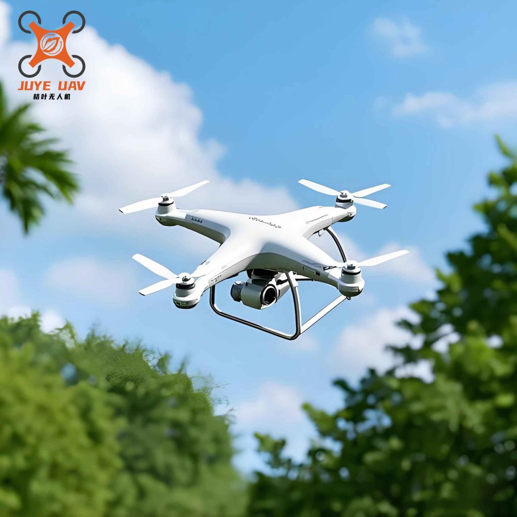
Figure: China UAV equipped with LiDAR sensor for autonomous navigation.
4. High-Level Planner
The high-level planner generates temporary target points in the UAV’s body frame at 10 Hz. It uses the precomputed global path from A* and a polar coordinate point cloud representation as input. The point cloud is processed as follows:
- Raw point cloud filtering: keep points within 10 m range, vertical field ±30°, horizontal field 120°.
- Polar gridding: divide horizontal range [-60°,+60°] into 12 sectors (10° each), vertical range [-30°,+30°] into 8 bins (7.5° each). Each cell stores the maximum normalized intensity.
- Flatten the 12×8 grid into a 96-dimensional vector and concatenate with UAV state (position, expected guide point).
The state space for the planner is st = [px, py, pz, pexp, Obsouter], where Obsouter is the flattened polar feature. The action is a 3D offset in the body frame. The reward function is:
$$ r = r_{\text{obs}} + r_{\text{action}} $$
$$ r_{\text{obs}} = \begin{cases} +100 & \text{if reached goal} \\ -60 & \text{if collision} \\ -k \cdot \text{dist} & \text{per step} \end{cases} $$
$$ r_{\text{action}} = -k_1 \Delta_{\text{goal}} $$
with k=0.1, k1=0.05. Training parameters: γ=0.999, H0=-3 (action dimension 3), learning rate 2×10⁻⁵, batch size 256, 15000 training steps. Table 2 shows performance comparisons.
| Planner | Training Steps | Inference Frequency (Hz) | Success Rate (%) | Obstacle Avoidance Rate (%) | Path Length (m) |
|---|---|---|---|---|---|
| SAC | 15000 | 20 | 100 | 95.8 | 1485 |
| SAC | 10000 | 10 | 98.3 | 87.5 | 1456 |
| DDPG | 15000 | 10 | 96.5 | 74.4 | 1487 |
| DDPG | 15000 | 20 | 96.7 | 76.5 | 1504 |
| SAC | 15000 | 10 | 100 | 95.1 | 1401 |
The SAC-trained planner achieves 100% success rate with 10 Hz inference frequency and shorter path lengths compared to DDPG. The frequency of 10 Hz allows better long-term planning without excessive replanning.
We also studied the impact of low-level controller accuracy on high-level performance, as shown in Table 3.
| Low-Level Position Error (m) | High-Level Success Rate (%) | Training Convergence Steps |
|---|---|---|
| 0.12 | 82.1 | 16700 |
| 0.09 | 94.5 | 10000 |
| 0.07 | 97.7 | 8200 |
Improved low-level precision directly enhances high-level success rate and accelerates convergence. This validates the two-layer cooperative design.
5. Experimental Validation
We conducted simulations in two different maps (200×110×110 m) with various obstacle configurations and starting/goal positions. The China UAV model matches the dynamics described earlier. SAC was used for both layers with optimal hyperparameters determined by sensitivity analysis. Hidden layer neuron number and learning rate were tuned: 256 neurons and learning rate 3×10⁻⁴ for low-level, and 256 neurons with learning rate 2×10⁻⁵ for high-level.
We compared our HRL-SAC approach against three baselines: (1) A* + MPC (traditional), (2) single-layer PPO, and (3) HRL-DDPG. Results are shown in Table 4.
| Method | Navigation Success Rate (%) | Obstacle Avoidance Rate (%) | Path Length (m) | Training Convergence Steps |
|---|---|---|---|---|
| A* + MPC | 85.3 | 82.1 | 1523 | N/A |
| PPO | 78.6 | 71.3 | 1587 | 29000 |
| HRL-DDPG | 91.2 | 83.5 | 1468 | 2400 + 9800 |
| HRL-SAC (Ours) | 97.7 | 91.8 | 1401 | 1500 + 8200 |
Our method achieves the highest success rate and obstacle avoidance rate, and the shortest average path length. The total training steps (1500 for low-level + 8200 for high-level) are significantly fewer than single-layer PPO. The maximum entropy of SAC improves exploration and policy robustness.
Sensitivity analysis on hidden layer neurons and learning rate for the high-level planner is summarized in Table 5.
| Neurons | Learning Rate | Convergence Steps | Position Error (m) |
|---|---|---|---|
| 64 | 3×10⁻⁴ | 9700 | 0.089 |
| 128 | 3×10⁻⁴ | 8700 | 0.074 |
| 256 | 3×10⁻⁴ | 8200 | 0.067 |
| 512 | 3×10⁻⁴ | 8000 | 0.065 |
256 neurons offer the best balance between performance and training time. For learning rate, Table 6 shows the results.
| Learning Rate | Neurons | Convergence Steps | Position Error (m) |
|---|---|---|---|
| 1×10⁻⁴ | 256 | 12900 | 0.066 |
| 3×10⁻⁴ | 256 | 8200 | 0.067 |
| 1×10⁻³ | 256 | 8100 | 0.085 |
The learning rate 3×10⁻⁴ gives the fastest convergence with acceptable error. These hyperparameters are adopted for all experiments.
The training reward curves for low-level and high-level controllers (not shown as figures due to prohibition of figure referencing) demonstrate stable convergence. The low-level controller reward reaches a plateau around step 2000, while the high-level planner converges near step 12000. The overall system exhibits strong robustness to sensor noise and dynamic obstacles.
6. Conclusion
We have developed a hierarchical reinforcement learning framework for China UAV autonomous navigation. By decoupling global path planning and local tracking, our system achieves high success rates (97.7%) and obstacle avoidance (91.8%) while maintaining short path lengths. The SAC algorithm with maximum entropy enhances exploration and policy stability. The asynchronous frequency matching (10 Hz planner, 150 Hz controller) ensures real-time performance. Sensitivity analysis confirms the optimal choice of network size and learning rate. This work provides a scalable solution for China UAV operations in complex environments. Future work will focus on online learning and real-world deployment to further improve adaptability.