
We present a novel disturbance-observer-based adaptive stochastic fuzzy model predictive control (DO-AFSMPC) framework for China UAV attitude stabilization under severe nonlinearities, multi-source disturbances, and parametric uncertainties. The proposed method integrates Takagi-Sugeno (T-S) fuzzy modeling, unscented Kalman filtering (UKF), disturbance observer (DO), and Q-learning optimization within a single predictive control architecture to achieve robust and accurate tracking performance. Extensive simulations demonstrate that our approach significantly outperforms conventional SMPC and adaptive fuzzy SMPC in terms of tracking accuracy, disturbance rejection, and model mismatch robustness, thereby providing a reliable solution for China UAV operations in complex environments.
1. Introduction
Quadrotor China UAV platforms have gained widespread adoption in both civilian and military domains due to their vertical take-off, hovering, and agile maneuverability. However, the inherent strong nonlinearity, under-actuation, and coupling dynamics, combined with external wind gusts, sensor noise, and parameter variations, pose significant challenges for attitude control. Traditional PID controllers often fail under aggressive maneuvers or heavy disturbances. Model predictive control (MPC) offers a promising alternative by handling constraints and optimizing future behavior, but its fixed-weight formulation limits adaptability. To address these issues, we propose a composite control strategy that combines random MPC, T-S fuzzy linearization, disturbance observer compensation, adaptive UKF state estimation, and Q-learning-based online weight tuning. This work aims to enhance the autonomy and robustness of China UAV attitude control systems.
2. Quadrotor Dynamics and Modeling
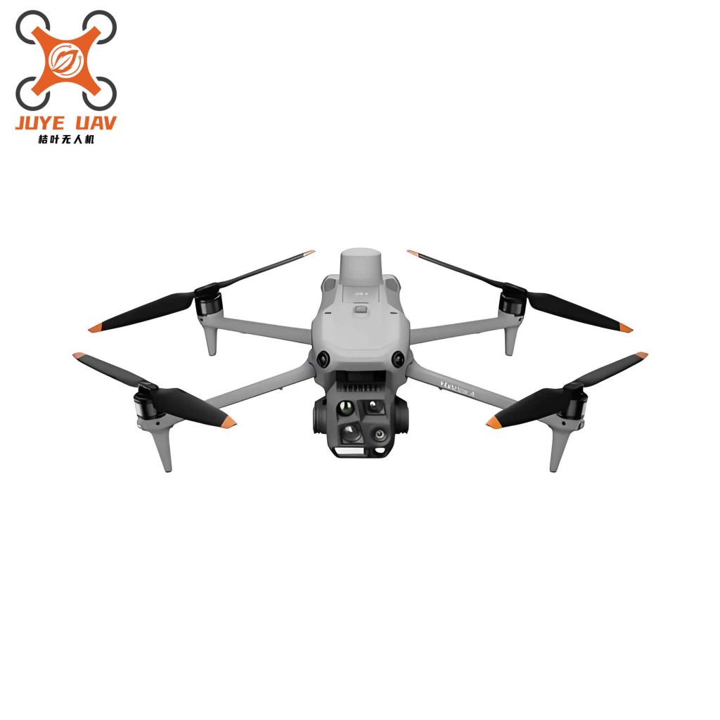
We consider an X-type quadrotor China UAV. The body-fixed frame B and inertial frame E are defined with Euler angles (roll $\phi$, pitch $\theta$, yaw $\psi$). The rotation matrix from B to E is given by:
$$
\mathbf{R}_E^B = \mathbf{R}_x(\phi)\mathbf{R}_y(\theta)\mathbf{R}_z(\psi)
$$
where
$$
\mathbf{R}_x(\phi)=\begin{bmatrix}1&0&0\\0&\cos\phi&-\sin\phi\\0&\sin\phi&\cos\phi\end{bmatrix},\quad
\mathbf{R}_y(\theta)=\begin{bmatrix}\cos\theta&0&\sin\theta\\0&1&0\\-\sin\theta&0&\cos\theta\end{bmatrix},\quad
\mathbf{R}_z(\psi)=\begin{bmatrix}\cos\psi&-\sin\psi&0\\\sin\psi&\cos\psi&0\\0&0&1\end{bmatrix}
$$
The attitude dynamics are derived from Newton-Euler equations:
$$
\begin{aligned}
\dot{\phi}&=p+q\sin\phi\tan\theta+r\cos\phi\tan\theta\\
\dot{\theta}&=q\cos\phi-r\sin\phi\\
\dot{\psi}&=\frac{q\sin\phi+r\cos\phi}{\cos\theta}\\
\dot{p}&=a_1 q r + b_1 u_1\\
\dot{q}&=a_2 p r + b_2 u_2\\
\dot{r}&=a_3 p q + b_3 u_3
\end{aligned}
$$
with $a_1=\frac{J_{yy}-J_{zz}}{J_{xx}}$, $a_2=\frac{J_{zz}-J_{xx}}{J_{yy}}$, $a_3=\frac{J_{xx}-J_{yy}}{J_{zz}}$, $b_1=\frac{1}{J_{xx}}$, $b_2=\frac{1}{J_{yy}}$, $b_3=\frac{1}{J_{zz}}$. The control inputs $u_1,u_2,u_3$ are related to rotor speeds via:
$$
\begin{bmatrix}u_1\\u_2\\u_3\end{bmatrix}=\begin{bmatrix}0&k_T l&0&-k_T l\\-k_T l&0&k_T l&0\\k_D&-k_D&k_D&-k_D\end{bmatrix}\begin{bmatrix}\omega_1^2\\\omega_2^2\\\omega_3^2\\\omega_4^2\end{bmatrix}
$$
We define state vector $\mathbf{x}=[\phi,\theta,\psi,p,q,r]^T$ and output $\mathbf{y}=[\phi,\theta,\psi]^T$. The system is expressed in state-space form:
$$
\begin{cases}
\dot{\mathbf{x}}=f(\mathbf{x},\mathbf{u})\\
\mathbf{y}=C\mathbf{x}
\end{cases}
$$
3. T-S Fuzzy Model Representation
To handle strong nonlinearities, we employ a T-S fuzzy model that decomposes the operating space into nine local linear models. The premise variables are roll and pitch angles. For each rule $i$, we have:
$$
\mathbf{x}_{k+1}=\mathbf{A}_i\mathbf{x}_k+\mathbf{B}_i\mathbf{u}_k+\mathbf{R}_i+\mathbf{d}_k
$$
where $\mathbf{A}_i$, $\mathbf{B}_i$ are Jacobians evaluated at operating points listed in Table 1. The overall fuzzy output is:
$$
\mathbf{x}_{k+1}=\sum_{i=1}^{N}\mu_i(z_k)(\mathbf{A}_i\mathbf{x}_k+\mathbf{B}_i\mathbf{u}_k+\mathbf{R}_i)+\mathbf{d}_k
$$
with Gaussian membership functions $\mu_i(z_k)=\frac{\exp(-\frac{(z_k-\bar{z}_i)^2}{2\sigma^2})}{\sum_{j}\exp(-\frac{(z_k-\bar{z}_j)^2}{2\sigma^2})}$.
| Rule | $\phi$ (deg) | $\theta$ (deg) | $\psi$ (deg) |
|---|---|---|---|
| 1 | -45 | -45 | 0 |
| 2 | -45 | 0 | 0 |
| 3 | -45 | 45 | 0 |
| 4 | 0 | -45 | 0 |
| 5 | 0 | 0 | 0 |
| 6 | 0 | 45 | 0 |
| 7 | 45 | -45 | 0 |
| 8 | 45 | 0 | 0 |
| 9 | 45 | 45 | 0 |
4. Stochastic Model Predictive Controller
We consider discrete-time stochastic system with process noise $\mathbf{w}_k$ and measurement noise $\mathbf{v}_k$:
$$
\mathbf{x}_{k+1}=\mathbf{A}\mathbf{x}_k+\mathbf{B}\mathbf{u}_k+\mathbf{w}_k,\quad \mathbf{y}_k=C\mathbf{x}_k+\mathbf{v}_k
$$
At each time $k$, we predict outputs over horizon $N_p$:
$$
\hat{\mathbf{Y}}_k=\mathbf{P}\mathbf{x}_k+\mathbf{H}\mathbf{U}_k
$$
where $\mathbf{P}=[C;CA;\dots;CA^{N_p}]^T$, $\mathbf{H}$ is the pulse response matrix. The cost function is:
$$
J=\hat{\mathbf{Y}}_k^T\mathbf{Q}\hat{\mathbf{Y}}_k+\mathbf{U}_k^T\mathbf{W}\mathbf{U}_k
$$
After substitution, we obtain quadratic programming:
$$
\min_{\mathbf{U}_k} \frac{1}{2}\mathbf{U}_k^T\mathbf{E}\mathbf{U}_k+\mathbf{F}^T\mathbf{U}_k
$$
with $\mathbf{E}=2(\mathbf{H}^T\mathbf{Q}\mathbf{H}+\mathbf{W})$, $\mathbf{F}=2\mathbf{H}^T\mathbf{Q}\mathbf{P}\mathbf{x}_k$. Input constraints and rate constraints are included:
$$
\mathbf{u}_{\min}\le\mathbf{u}\le\mathbf{u}_{\max},\quad \Delta\mathbf{u}_{\min}\le\Delta\mathbf{u}\le\Delta\mathbf{u}_{\max}
$$
5. Disturbance Observer Design
To compensate unknown disturbances $\mathbf{d}_k$, we design a disturbance observer:
$$
\begin{aligned}
\mathbf{d}_{k+1} &= \mathbf{F}\mathbf{x}_k + \mathbf{z}_k \\
\mathbf{z}_{k+1} &= \mathbf{z}_k + \mathbf{F}((\mathbf{A}-\mathbf{I})\mathbf{x}_k+\mathbf{B}\mathbf{u}_k+\mathbf{R}_i+\mathbf{F}^{-1}\mathbf{z}_k)
\end{aligned}
$$
The observer gain $\mathbf{F}$ is chosen such that the estimation error dynamics are stable. The control input is then corrected:
$$
\mathbf{u}_k = \mathbf{u}_{c,k} – \mathbf{F}_d\hat{\mathbf{d}}_k
$$
6. Adaptive Unscented Kalman Filter
We employ an adaptive UKF to estimate system states and suppress measurement noise. The sigma points are generated as:
$$
\begin{aligned}
\mathcal{X}_{k-1}^{(0)} &= \hat{\mathbf{x}}_{k-1} \\
\mathcal{X}_{k-1}^{(i)} &= \hat{\mathbf{x}}_{k-1} + \sqrt{(n+\lambda)\mathbf{P}_{k-1}},\quad i=1,\dots,n \\
\mathcal{X}_{k-1}^{(i+n)} &= \hat{\mathbf{x}}_{k-1} – \sqrt{(n+\lambda)\mathbf{P}_{k-1}},\quad i=1,\dots,n
\end{aligned}
$$
After propagation through the nonlinear dynamics, we compute predicted mean and covariance, then update with measurement. The measurement noise covariance is adaptively adjusted:
$$
\mathbf{P}_{zz,k} = (1-\beta)\mathbf{P}_{zz,k-1} + \beta(\mathbf{z}_k-\hat{\mathbf{z}}_k)(\mathbf{z}_k-\hat{\mathbf{z}}_k)^T
$$
This adaptive mechanism improves robustness under varying noise levels, which is critical for China UAV operating in real-world environments.
7. Q-learning Online Weight Optimization
We formulate the MPC weight tuning as a Markov decision process. The state is defined by tracking error and its derivative:
$$
\mathbf{s}_k = \begin{bmatrix}e_k & \dot{e}_k\end{bmatrix}^T
$$
The action space consists of three discrete actions: increase weight, decrease weight, or keep current. The reward function combines tracking performance, control smoothness, and error improvement:
$$
r_k = w_1 r_t + w_2 r_s + w_3 r_i + r_v + r_p
$$
Q-values are updated as:
$$
Q(s,a) \leftarrow Q(s,a) + \alpha \left[r + \gamma \max_{a’} Q(s’,a’) – Q(s,a)\right]
$$
The learned policy dynamically adjusts the MPC weight matrix $\mathbf{W}$, balancing tracking accuracy and control effort. This allows the China UAV to adapt to changing flight conditions without manual retuning.
8. Stability Analysis
We consider the Lyapunov function:
$$
\mathcal{V}(k) = \mathbf{e}_k^T \mathbf{P} \mathbf{e}_k + J^\ast(k)
$$
where $\mathbf{e}_k=\mathbf{x}_k-\mathbf{x}_{r,k}$. Under the combined effect of disturbance observer and UKF, the state error dynamics are asymptotically stable, satisfying:
$$
\mathbf{e}_{k+1}^T \mathbf{P} \mathbf{e}_{k+1} – \mathbf{e}_k^T \mathbf{P} \mathbf{e}_k \le -\mathbf{e}_k^T \mathbf{Q}_e \mathbf{e}_k
$$
For the Q-learning optimized MPC, the cost function decreases monotonically: $J^\ast(k+1) \le J^\ast(k) – \ell(\mathbf{x}_k,\mathbf{u}_k)$. Therefore, $\Delta \mathcal{V}(k) \le 0$, proving asymptotic stability of the closed-loop system for China UAV attitude control.
9. Simulation Results
We conducted extensive simulations to compare DO-AFSMPC with conventional SMPC and adaptive fuzzy SMPC (AFSMPC). The China UAV model parameters are listed in Table 2.
| Parameter | Value |
|---|---|
| Mass | 1.545 kg |
| Arm length | 0.255 m |
| Thrust coefficient $k_T$ | 5.84e-6 N/(rad/s)^2 |
| Drag coefficient $k_D$ | 1.168e-7 N/(rad/s)^2 |
| $J_{xx}$ | 0.029 kg·m² |
| $J_{yy}$ | 0.029 kg·m² |
| $J_{zz}$ | 0.055 kg·m² |
| $\omega_{\min}$ | 1805 rad/s |
| $\omega_{\max}$ | 11100 rad/s |
The reference trajectories are:
$$
\phi_r(k)=\cos(0.2k-0.1),\quad \theta_r(k)=\sin(0.05\pi k),\quad \psi_r(k)=\cos(0.2k-0.1)
$$
We first tested the effect of prediction horizon. Results show that shorter $N_p$ gives faster convergence but larger steady-state error. Our adaptive strategy dynamically adjusts $N_p$ based on tracking error, balancing performance and computational load.
Under sinusoidal disturbances (amplitude 0.1, frequency 0.0318 Hz), DO-AFSMPC achieved the smallest attitude oscillations. The root mean square error (RMSE) for roll angle reduced by 12% compared to AFSMPC, as summarized in Table 3.
| Controller | RMSE $\phi$ | RMSE $\theta$ | RMSE $\psi$ |
|---|---|---|---|
| SMPC | 0.0412 | 0.0518 | 0.0453 |
| AFSMPC | 0.0307 | 0.0377 | 0.0326 |
| DO-AFSMPC | 0.0269 | 0.0291 | 0.0301 |
Model mismatch tests with $\pm20\%$ inertia variations further confirmed the robustness of DO-AFSMPC. The control inputs were smoother with negligible overshoot, unlike SMPC which exhibited chattering. Ablation studies validated that each component (Q-learning, UKF, DO) contributes significantly to the overall performance. The cumulative reward of the full algorithm was consistently higher, and the tracking error converged faster and remained lower than any ablated version.
Hyperparameter sensitivity analysis for Q-learning showed that learning rate $\alpha\in[0.2,0.4]$ and discount factor $\gamma\in[0.55,0.6]$ yield the best convergence and stability. Taken together, these results highlight the superior capability of our DO-AFSMPC for China UAV attitude control in challenging environments.
10. Conclusion
We have developed a disturbance-observer-based adaptive stochastic fuzzy model predictive control method that integrates Q-learning and unscented Kalman filtering for China UAV attitude regulation. The T-S fuzzy model linearizes the nonlinear dynamics into multiple local models, enabling efficient MPC computation. The disturbance observer compensates external wind and model mismatch, while the adaptive UKF provides reliable state estimates under measurement noise. Q-learning online optimizes the MPC weight matrix, allowing the controller to self-tune for varying flight conditions. Lyapunov stability analysis guarantees closed-loop convergence. Simulation results confirm that DO-AFSMPC significantly outperforms conventional SMPC and AFSMPC in tracking accuracy, disturbance rejection, and robustness against parameter variations. Future work will focus on hardware-in-the-loop validation on Pixhawk flight controllers to bridge the gap between simulation and real-world deployment for China UAV systems.