
River flow velocity and discharge are fundamental parameters for water resource management, flood control, and ecological monitoring. Traditional measurement instruments such as rotors, electromagnetic current meters, and Acoustic Doppler Current Profilers (ADCP) provide reliable accuracy but often require manual deployment or boat-based operations, leading to high safety risks, cumbersome procedures, and limitations under complex flow conditions. In recent years, the integration of unmanned aerial vehicles (UAVs) with video processing technologies has enabled non-contact flow measurement, leveraging surface texture or floating object displacement to infer surface velocities. This approach, especially when applied with China UAV platforms, offers advantages in portability, safety, and deployment flexibility. However, existing methods still face challenges such as unstable feature points, difficult image distortion correction, and significant pixel-scale mapping errors. In particular, the accuracy of velocity inversion is compromised by inadequate orthorectification, lens distortion, and attitude variations of the UAV. Recognizing the increasing demand for rapid and precise flow measurement in water-scarce regions such as Hebei Province, this study systematically improves the UAV-based image-tracking flow measurement method. By optimizing flight parameters, enhancing feature tracking algorithms, and establishing a precise scale conversion model, we significantly boost the accuracy and reliability of surface velocity measurements. Field experiments were conducted on a typical river reach in Hebei Province using a China UAV platform, and the results were validated against ADCP measurements. This work provides a reusable technical pathway for regional hydrological monitoring.
1. Improved UAV Image-Based Flow Measurement Method
1.1 Technical Framework
The proposed improvement consists of three core components: data acquisition optimization, feature point tracking algorithm enhancement, and flow velocity calculation model refinement. The overall workflow integrates these components to produce high-quality surface velocity fields from UAV video sequences.
1.2 Data Acquisition Optimization
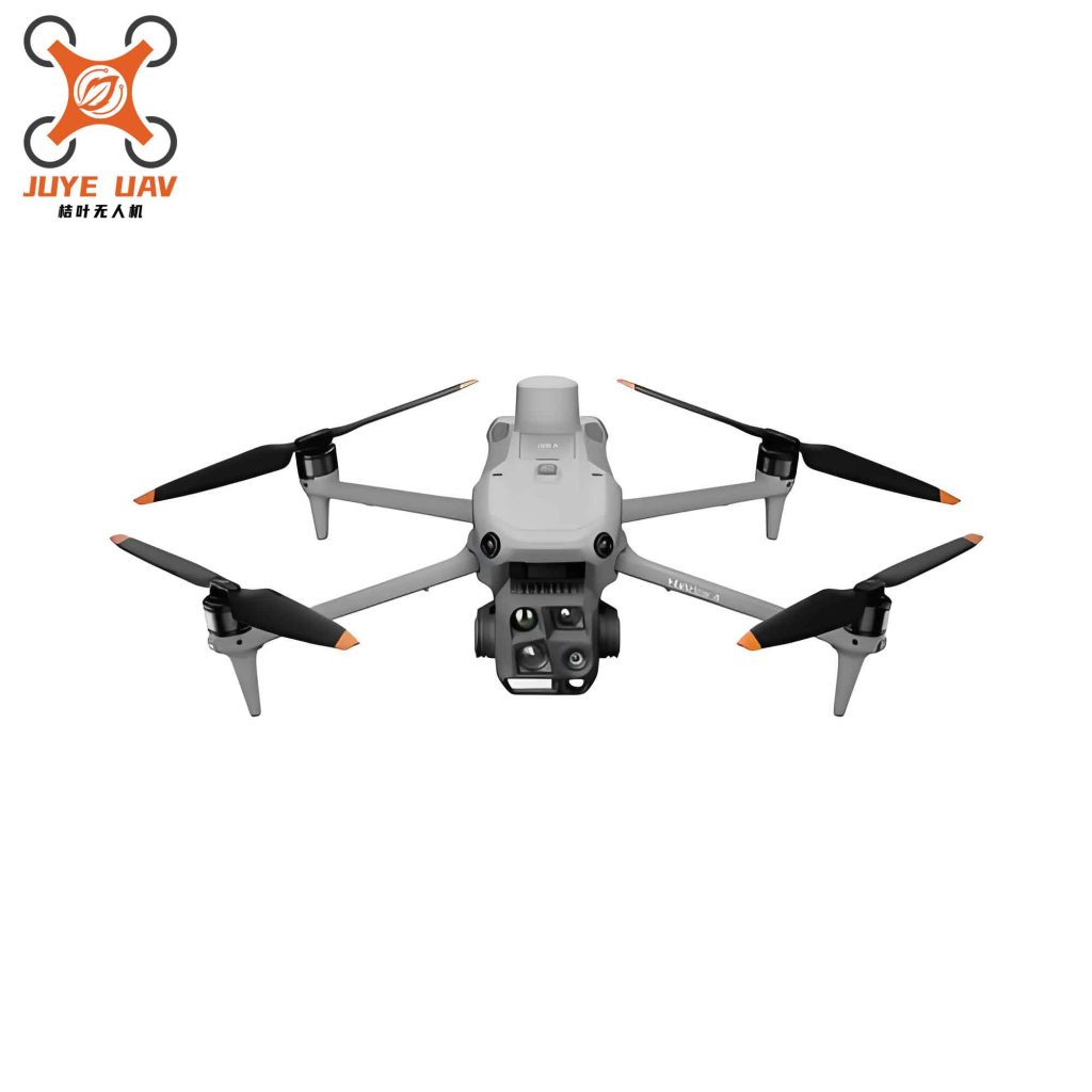
To minimize the influence of distortion, tilt, and platform vibration on feature extraction and velocity inversion, we designed a standardized China UAV flight procedure. The flying platform is the DJI Phantom 4 RTK, which outputs real-time POS (Position and Orientation System) data to improve exterior orientation accuracy for orthorectification and scale conversion. The camera resolution is 3840×2160 at a frame rate of 30 fps, enabling clear recording of surface texture and drift trajectories. The flight altitude was maintained at 50 m with the lens pointing vertically downward (90°) to suppress perspective distortion, achieving a ground sampling distance (GSD) of approximately 2.7 cm/pixel. This setting balances feature identification and river coverage. The flight path was straight with constant speed, and a three-axis gimbal stabilized the camera. Flights were scheduled during low-wind conditions and away from strong reflection areas to ensure continuous and stable image sequences.
For accurate scale mapping from pixel displacement to real-world displacement, four ground control points (GCPs) were deployed on both riverbanks. Their coordinates were measured using a Huace i80 RTK system with a horizontal accuracy better than ±2 cm. PVC or checkerboard targets were used to enhance corner detection. The combined adjustment of GCP and POS data effectively reduces scale errors, keeping the velocity conversion deviation within an acceptable range.
1.3 Improved KLT Feature Point Tracking Algorithm
The Kanade-Lucas-Tomasi (KLT) algorithm is a classical sparse optical flow method for feature point tracking. It relies on grayscale consistency, local gradient properties, and small displacement assumptions to match points across frames. However, on water surfaces, weak texture, strong reflection, and drifting targets often lead to tracking failures. We therefore propose an enhanced KLT framework tailored for water surface applications.
1.3.1 Adaptive Feature Point Extraction
We used an improved Shi-Tomasi corner detector, where the corner response function \( R \) is defined as:
$$ R = \min(\lambda_1, \lambda_2) $$
Here \( R \) is the corner response value, and \( \lambda_1, \lambda_2 \) are the eigenvalues of the grayscale gradient covariance matrix in a local window. The threshold is adaptively adjusted based on water surface texture characteristics, ensuring stable feature points even in low-texture areas.
1.3.2 Pyramid Optical Flow Tracking
A three-layer image pyramid was constructed. Tracking starts at the lowest resolution layer and progressively refines to the original resolution. This multi-resolution strategy effectively handles large displacements of feature points, improving algorithm robustness.
1.3.3 Bidirectional Tracking Verification
We introduced a forward-backward verification mechanism. The forward tracking step is:
$$ P_t = KLT(P_{t-1}) $$
The backward verification step is:
$$ P’_{t-1} = KLT^{-1}(P_t) $$
Acceptance condition:
$$ \|P_{t-1} – P’_{t-1}\| < \epsilon $$
where \( P_t, P_{t-1} \) are image coordinates of the feature point at times \( t \) and \( t-1 \); \( P’_{t-1} \) is the estimated coordinate from backward tracking; \( KLT \) is the forward tracking function; \( KLT^{-1} \) is the backward tracking function; and \( \epsilon \) is a preset threshold (typically 1–2 pixels). This mechanism effectively eliminates false matches and enhances tracking stability.
1.4 Velocity Calculation and Scale Conversion Model
1.4.1 Camera Calibration and Distortion Correction
Zhang’s calibration method was employed to determine intrinsic camera parameters and correct lens distortion. The distortion correction model is:
$$ x_{\text{corrected}} = x(1 + k_1 r^2 + k_2 r^4 + k_3 r^6) + 2p_1 xy + p_2(r^2 + 2x^2) $$
$$ y_{\text{corrected}} = y(1 + k_1 r^2 + k_2 r^4 + k_3 r^6) + 2p_2 xy + p_1(r^2 + 2y^2) $$
Here \( x, y \) are the original distorted pixel coordinates; \( x_{\text{corrected}}, y_{\text{corrected}} \) are the corrected coordinates; \( r \) is the radial distance; \( k_1, k_2, k_3 \) are radial distortion coefficients; and \( p_1, p_2 \) are tangential distortion coefficients.
1.4.2 Spatial Scale Conversion
Using ground control points, we solved for the homography matrix \( \mathbf{H} \) via direct linear transformation to establish the relationship between image coordinates and real-world coordinates:
$$ \begin{bmatrix} X \\ Y \\ 1 \end{bmatrix} = \mathbf{H} \times \begin{bmatrix} u \\ v \\ 1 \end{bmatrix} $$
where \( u, v \) are pixel coordinates in the image; \( X, Y \) are plane coordinates in the real world. Considering water surface fluctuations and UAV attitude variations, we introduced a scale correction factor \( k \):
$$ k = \frac{H_{\text{nominal}}}{H_{\text{actual}}} $$
where \( H_{\text{actual}} \) is the actual height of the UAV above the water surface, and \( H_{\text{nominal}} \) is the nominal flight altitude.
1.4.3 Surface Velocity Calculation
The surface velocity \( V \) is computed from the actual displacement \( \Delta S \) of a feature point over a time interval \( \Delta t \):
$$ V = \frac{\Delta S}{\Delta t} $$
Here \( V \) is the surface velocity (m/s), \( \Delta t \) is the inverse of the video frame rate, and \( \Delta S \) is derived from the difference in real-world coordinates.
2. Case Study and Application Analysis
2.1 Study Area and Data Acquisition
The study area is located in the middle reach of the Hutuo River near Shijiazhuang City, Hebei Province, China. This region has a typical temperate continental monsoon climate with significant seasonal hydrological variations. The river reach is a plain-type gentle slope with a medium-to-fine sand bed, relatively uniform cross-section, average width of about 60 m, average depth of about 1.5 m, and surface velocities ranging from 0.3 to 1.2 m/s during the measurement period. The water surface exhibited adequate texture for image tracking.
Field data were collected on July 15, 2023, from 10:00–12:00 under clear skies and low wind (2–3 Beaufort), ensuring stable flow conditions. A China UAV (DJI Phantom 4 RTK) was flown along a perpendicular flight line to capture 2 minutes of continuous 4K video at 30 fps. Table 1 summarizes the flight parameters and data acquisition details. Simultaneously, an ADCP was used for boat-mounted cross-section measurements, acquiring five valid sets of velocity data for validation.
| Parameter Category | Specific Parameter | Remarks |
|---|---|---|
| Flight Platform | DJI Phantom 4 RTK | Built-in high-precision GNSS module |
| Flight Altitude | 50 m | Vertical height above water surface |
| Lens Angle | 90° (vertical downward) | Nadir shooting |
| Frame Rate | 30 fps | 30 frames per second |
| Resolution | 3840×2160 pixels | 4K ultra-high definition |
| Ground Sampling Distance (GSD) | 2.7 cm/pixel | Theoretical value |
| Video Duration | 2 min | Effective measurement time |
| Number of Control Points | 4 | Symmetric deployment on both banks |
2.2 Experimental Design and Evaluation Metrics
To validate the performance of the improved KLT algorithm for UAV-based surface velocity inversion, we compared it with the traditional KLT method. The traditional method uses a fixed threshold for feature extraction, lacks pyramid strategies and bidirectional verification, and thus suffers from drift and false tracking under weak texture or strong reflection. The improved method incorporates adaptive threshold, multi-resolution pyramid, bidirectional verification, and flow field smoothing. Both methods were applied to the same video sequence, and ADCP measurements served as ground truth. Evaluation metrics include tracking success rate, average pixel error, stability coefficient, mean absolute error (MAE), root mean square error (RMSE), coefficient of determination (\( R^2 \)), Nash-Sutcliffe Efficiency (NSE), and mean relative error (MRE).
2.3 Results Analysis
2.3.1 Feature Point Tracking Performance
Table 2 compares the tracking performance between the traditional KLT and the improved KLT. Although the improved method extracted slightly fewer initial feature points (682 vs. 735), the number of effectively tracked points increased significantly from 412 to 593. The tracking success rate improved from 56.1% to 87.0%, and the average pixel error decreased by 57.1% (from 2.8 to 1.2 pixels). The stability coefficient increased from 0.71 to 0.92, demonstrating enhanced robustness against reflection disturbances and sparse texture.
| Evaluation Index | Traditional KLT | Improved KLT | Improvement |
|---|---|---|---|
| Initial Feature Points | 735 | 682 | -7.2% |
| Effectively Tracked Points | 412 | 593 | +43.9% |
| Tracking Success Rate (%) | 56.1 | 87.0 | +30.9% |
| Average Pixel Error (pixels) | 2.8 | 1.2 | -57.1% |
| Stability Coefficient | 0.71 | 0.92 | +29.6% |
2.3.2 Surface Velocity Field Spatial Distribution
The derived velocity field shows that the highest velocities (1.1–1.2 m/s) occur in the central channel, gradually decreasing to 0.3–0.5 m/s near the banks. This pattern matches the typical velocity distribution in open-channel flow. The vector directions are consistent with the main stream direction, with no anomalous perturbations, confirming the stability of feature tracking and the physical reasonableness of the reconstructed flow field.
Comparison of cross-section velocity profiles (Figure 5 – not included) indicates that the improved KLT inversion closely matches the ADCP measured curve, especially in the main flow region (15–45 m). In contrast, the traditional KLT method overestimates velocities in the central channel, likely due to false matches and directional deviations. This further validates the advantage of the improved algorithm in flow field reconstruction.
2.3.3 Cross-Section Average Velocity Comparison
Table 3 lists the five sets of cross-section average velocities measured by ADCP, the improved KLT method, and the traditional KLT method. The relative errors of the improved method range from 3.4% to 4.4%, with an average of 3.8%, significantly lower than the traditional method’s average of 11.3%. The traditional method consistently overestimates, indicating a systematic bias caused by poor feature verification.
| Measurement | ADCP (m/s) | Improved KLT (m/s) | Relative Error (%) | Traditional KLT (m/s) | Relative Error (%) |
|---|---|---|---|---|---|
| 1 | 0.82 | 0.79 | 3.7 | 0.91 | 11.0 |
| 2 | 0.88 | 0.85 | 3.4 | 0.98 | 11.4 |
| 3 | 0.79 | 0.76 | 3.8 | 0.88 | 11.4 |
| 4 | 0.85 | 0.82 | 3.5 | 0.94 | 10.6 |
| 5 | 0.91 | 0.87 | 4.4 | 1.02 | 12.1 |
| Average | 0.85 | 0.82 | 3.8 | 0.95 | 11.3 |
2.3.4 Accuracy Validation and Error Analysis
The mean absolute error (MAE) was calculated as:
$$ \text{MAE} = \frac{1}{n} \sum_{i=1}^{n} |V_{\text{obs}}^i – V_{\text{pred}}^i| $$
where \( n \) is the number of samples, \( V_{\text{obs}}^i \) is the ADCP measured velocity, and \( V_{\text{pred}}^i \) is the UAV-derived velocity. Table 4 summarizes the accuracy metrics. The improved method achieves an MAE of 0.043 m/s, RMSE of 0.052 m/s, \( R^2 \) of 0.93, NSE of 0.90, and MRE of 5.2%. All these values satisfy the requirements of the Chinese Hydrometry Standard (allowable error <10% for surface velocity). In contrast, the traditional method yields MRE of 12.8%, exceeding the standard. The high NSE (0.90) indicates excellent agreement between predicted and observed values.
| Accuracy Metric | Improved Method | Traditional Method | Allowable Error Standard |
|---|---|---|---|
| MAE (m/s) | 0.043 | 0.109 | <0.10 |
| RMSE (m/s) | 0.052 | 0.135 | <0.15 |
| \( R^2 \) | 0.93 | 0.78 | >0.85 |
| NSE | 0.90 | 0.72 | >0.80 |
| MRE (%) | 5.2 | 12.8 | <10% |
3. Conclusion
This study systematically addresses the limitations of UAV-based image velocimetry, including sparse features, reflection interference, and tracking drift. We proposed an improved KLT velocity inversion framework and validated it using field data from the Hutuo River in Hebei Province. The adaptive feature extraction strategy effectively identifies robust features even on low-texture water surfaces, raising the tracking success rate from 56.1% to 87.0%. The combination of pyramid optical flow and bidirectional verification reduces the average pixel error from 2.8 to 1.2 pixels. The spatial conversion model with a scale correction factor compensates for geometric errors caused by water surface fluctuations. Overall, the improved method achieves a mean relative error of only 5.2% when compared with ADCP measurements, significantly better than the 12.8% of the traditional method, and fully meets the Chinese standard for surface velocity measurement. The enhanced robustness and engineering adaptability make this approach a reliable technical support for non-contact flow monitoring using China UAV platforms. Future work will extend the validation to multiple flow conditions and river morphologies to further assess the method’s generalizability.