
The mesmerizing spectacle of a formation drone light show represents a pinnacle of coordinated aerial robotics. Hundreds, sometimes thousands, of unmanned aerial vehicles (UAVs) move in perfect harmony, painting intricate, dynamic shapes against the night sky. Behind this visual poetry lies a formidable control engineering challenge: ensuring each drone maintains its precise position within the evolving formation despite inevitable real-world disruptions. These disruptions—gusts of wind, manufacturing variances leading to parameter uncertainties, unmodeled aerodynamic couplings between closely flying drones, and the wear-and-tear of actuators—continuously threaten to distort the intended pattern or, worse, cause mid-air collisions. This article delves into an advanced control methodology designed to empower formation drone light shows with exceptional robustness, precision, and safety, guaranteeing a flawless performance every time.
The Core Challenge: Precision Under Uncertainty
The fundamental task in a formation drone light show is trajectory tracking with inter-agent coordination. Typically organized in a leader-follower structure, a designated leader drone executes the master trajectory, while follower drones must maintain specific geometric offsets relative to it. For a triangular formation, these offsets are defined as desired longitudinal and lateral distances within a moving coordinate frame attached to the leader.
Let the leader’s planar position and heading be $(x_L, y_L)$ and $\varphi_L$, respectively. For a follower $i$, the desired position in the global inertial frame is given by:
$$
\begin{aligned}
x_{gr}^{Fi} &= x_L – L_{x}^{Fi} \cos \varphi_L + L_{y}^{Fi} \sin \varphi_L, \\
y_{gr}^{Fi} &= y_L – L_{x}^{Fi} \sin \varphi_L – L_{y}^{Fi} \cos \varphi_L.
\end{aligned}
$$
Here, $L_{x}^{Fi}$ and $L_{y}^{Fi}$ are the desired formation offsets transformed into the inertial frame. The core control error for each follower is therefore:
$$
e_x^{Fi} = x_{gr}^{Fi} – x^{Fi}, \quad e_y^{Fi} = y_{gr}^{Fi} – y^{Fi}.
$$
The dynamics of a follower drone, accounting for real-world effects, can be modeled as:
$$
\begin{aligned}
\dot{x}^{Fi} &= v^{Fi} \cos \varphi^{Fi}, \\
\dot{y}^{Fi} &= v^{Fi} \sin \varphi^{Fi}, \\
\dot{v}^{Fi} &= (1 – \kappa_a) a^{Fi} + d_{wind1}^{Fi}, \\
\dot{\varphi}^{Fi} &= (1 – \kappa_p) p^{Fi} + d_{wind2}^{Fi}.
\end{aligned}
$$
Here, $a^{Fi}$ and $p^{Fi}$ are the acceleration and heading rate control inputs. The terms $\kappa_a, \kappa_p \in [0, 0.8)$ represent actuator fault coefficients (partial loss of effectiveness), and $d_{wind}^{Fi}$ account for external wind disturbances. Differentiating the error dynamics and consolidating unknown terms leads to a second-order system for each axis:
$$
\ddot{e}_j^{Fi} = u_j^{Fi} + D_j^{Fi}, \quad j \in \{x, y\}.
$$
The virtual control $u_j^{Fi}$ is a function of the actual drone commands. Crucially, the lumped disturbance $D_j^{Fi}$ encapsulates a multitude of challenging effects:
$$ D_j^{Fi} = \text{(Leader maneuvering terms)} + \text{(Wind disturbances)} – \kappa_a a^{Fi} \text{ or } \kappa_p p^{Fi} v^{Fi} \text{ terms}. $$
This term is complex, time-varying, and incorporates both external disturbances and internal faults. The primary control objectives are: 1) Force $e_j^{Fi}(t)$ to converge to zero (precise formation keeping). 2) Ensure the convergence process respects strict transient bounds to prevent collisions. 3) Achieve these goals despite the unknown, high-order time-varying disturbance $D_j^{Fi}$.
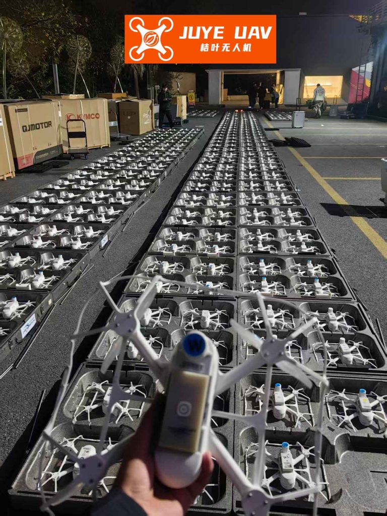
As visualized, the complexity of a formation drone light show demands that these control objectives are met simultaneously for every agent in the swarm. A single drone’s deviation can break the illusion.
Pillar I: Prescribed Performance without Prior Knowledge
To guarantee safety during transient maneuvers, such as when the formation dynamically reconfigures, we enforce that the tracking error remains within a designer-specified performance envelope at all times:
$$ -\rho_j(t) < e_j^{Fi}(t) < \rho_j(t). $$
The performance function $\rho_j(t)$ defines this evolving envelope. Traditional exponential performance functions, $\rho(t) = (\rho_0 – \rho_\infty)e^{-lt} + \rho_\infty$, require knowledge of the initial error bound $|e(0)| < \rho_0$, which is often impractical for a formation drone light show starting from arbitrary deployment positions.
We overcome this limitation by introducing a novel performance function based on the hyperbolic cotangent:
$$ \rho_j(t) = \coth(k_j t + l_j) – 1 + \rho_{j\infty}. $$
Here, $\rho_{j\infty}>0$ is the ultimate steady-state error bound, $k_j>0$ governs the convergence rate, and $l_j>0$ is a small positive constant. This function’s key advantage is its property: $\lim_{l_j \to 0^+} \rho_j(0) = +\infty$. By choosing a sufficiently small $l_j$, we can ensure $|e_j^{Fi}(0)| < \rho_j(0)$ for any finite initial error, effectively removing the need for prior knowledge of the initial condition. The function is strictly decreasing and converges to $\rho_{j\infty}$.
To transform this constrained problem into an unconstrained one, we define a normalized error and a transformed error:
$$ \tilde{e}_j(t) = \frac{e_j^{Fi}(t)}{\rho_j(t)}, \quad \varepsilon_j(t) = \frac{1}{2} \ln \left( \frac{1 + \tilde{e}_j(t)}{1 – \tilde{e}_j(t)} \right). $$
The mapping between $\tilde{e}_j$ and $\varepsilon_j$ is a bijective hyperbolic tangent function. Crucially, ensuring the boundedness of $\varepsilon_j(t)$ automatically guarantees $|\tilde{e}_j(t)| < 1$, which is equivalent to the original performance constraint $|e_j^{Fi}(t)| < \rho_j(t)$. Therefore, the control objective becomes the stabilization of the transformed error dynamics $\varepsilon_j(t)$.
Pillar II: Estimating High-Order Uncertainties with GPIO
The lumped disturbance $D_j^{Fi}$ in the error dynamics is not merely constant or slowly varying. Due to the combination of fault effects, wind gusts, and leader maneuver dynamics, it can exhibit high-order time-varying behavior. A simple disturbance observer may not track it accurately enough. We employ a Generalized Proportional Integral Observer (GPIO) for precise estimation.
We assume the disturbance $D_j^{Fi}$ has a bounded second derivative. For the x-axis channel of follower $i$, the GPIO is designed as:
$$
\begin{aligned}
\dot{z}_{x1}^{Fi} &= z_{x2}^{Fi} – \beta_{x1}^{Fi}(z_{x1}^{Fi} – e_x^{Fi}), \\
\dot{z}_{x2}^{Fi} &= z_{x3}^{Fi} – \beta_{x2}^{Fi}(z_{x1}^{Fi} – e_x^{Fi}) + u_x^{Fi}, \\
\dot{z}_{x3}^{Fi} &= z_{x4}^{Fi} – \beta_{x3}^{Fi}(z_{x1}^{Fi} – e_x^{Fi}), \\
\dot{z}_{x4}^{Fi} &= -\beta_{x4}^{Fi}(z_{x1}^{Fi} – e_x^{Fi}).
\end{aligned}
$$
The estimates are provided by: $\hat{\dot{e}}_x^{Fi} = z_{x2}^{Fi}$ (error derivative) and $\hat{D}_x^{Fi} = z_{x3}^{Fi}$ (lumped disturbance). The gains $\beta_{x1}^{Fi}, …, \beta_{x4}^{Fi}$ are chosen such that the observer’s characteristic polynomial $s^4 + \beta_{x1}^{Fi}s^3 + \beta_{x2}^{Fi}s^2 + \beta_{x3}^{Fi}s + \beta_{x4}^{Fi}$ is Hurwitz. An identical observer runs for the y-axis channel. This GPIO structure extends the estimation capability beyond the disturbance itself ($D$) to its derivative ($\dot{D}$), housed in the state $z_{x4}^{Fi}$, enabling accurate tracking of higher-order variations critical for a dynamic formation drone light show.
The Composite Control Law
Integrating the prescribed performance transformation and the GPIO estimates, we construct an active disturbance rejection controller. The goal is to stabilize the transformed error $\varepsilon_j$, whose second-order dynamics are derived as:
$$ \ddot{\varepsilon}_j = n_j (u_j^{Fi} + D_j^{Fi}) + f(\cdot), $$
where $n_j = 1/[\rho_j (1+\tilde{e}_j)(1-\tilde{e}_j)] > 0$ and $f(\cdot)$ contains terms involving known functions of $\rho_j$, $\tilde{e}_j$, and their derivatives.
The composite control law is designed to actively cancel the disturbance and impose desired dynamics on $\varepsilon_j$:
$$
u_j^{Fi} = -\frac{k_p}{n_j} \varepsilon_j – \frac{k_d}{n_j} \dot{\varepsilon}_j – \frac{\dot{n}_j}{n_j}(\hat{\dot{e}}_j^{Fi} – \dot{\tilde{e}}_j \rho_j) + \dot{\tilde{e}}_j \dot{\rho}_j + \tilde{e}_j \ddot{\rho}_j – \hat{D}_j^{Fi}.
$$
Here, $k_p, k_d > 0$ are controller gains. The terms $-\hat{D}_j^{Fi}$ provide direct feedforward cancellation of the estimated lumped disturbance. The remaining terms compensate for the nonlinear transformation and enforce the target closed-loop dynamics $\ddot{\varepsilon}_j + k_d \dot{\varepsilon}_j + k_p \varepsilon_j \approx 0$ for the transformed error.
Finally, the virtual control commands $u_x^{Fi}, u_y^{Fi}$ are converted back into the actual drone acceleration and heading rate commands via the inverse transformation:
$$
\begin{bmatrix} a^{Fi} \\ p^{Fi} \end{bmatrix} =
\begin{bmatrix}
-\cos \varphi^{Fi} & -\sin \varphi^{Fi} \\
\frac{\sin \varphi^{Fi}}{v^{Fi}} & -\frac{\cos \varphi^{Fi}}{v^{Fi}}
\end{bmatrix}
\begin{bmatrix} u_x^{Fi} \\ u_y^{Fi} \end{bmatrix}.
$$
Stability and Performance Guarantees
The closed-loop system’s stability can be analyzed by considering the combined state of estimation errors and the transformed tracking error. Defining the observer error states as $e_{j1} = z_{j1} – e_j$, $e_{j2} = \hat{\dot{e}}_j – \dot{e}_j$, $e_{j3} = \hat{D}_j – D_j$, $e_{j4} = \hat{\dot{D}}_j – \dot{D}_j$, their dynamics coupled with the transformed error dynamics form an augmented system:
$$ \dot{\mathbf{E}}_j = \mathbf{A}_j \mathbf{E}_j + \mathbf{B} \ddot{D}_j^{Fi}, $$
where $\mathbf{E}_j = [e_{j1}, e_{j2}, e_{j3}, e_{j4}, \varepsilon_j, \dot{\varepsilon}_j]^T$. The matrix $\mathbf{A}_j$ is Hurwitz due to the proper selection of observer and controller gains. Given the assumption that $\ddot{D}_j^{Fi}$ is bounded and tends to zero as the formation maneuver settles, the entire augmented error system $\mathbf{E}_j$ is globally uniformly ultimately bounded. Furthermore, the estimation errors $e_{j2}, e_{j3}$ converge to a small neighborhood of zero.
This guarantees:
- Convergence: The transformed error $\varepsilon_j(t)$ converges to near zero, implying the original tracking error $e_j^{Fi}(t)$ converges to a small vicinity of zero (ultimately bounded by $\rho_{j\infty}$).
- Prescribed Performance: Throughout the entire response, the tracking error $e_j^{Fi}(t)$ is strictly maintained within the predefined envelope $(-\rho_j(t), \rho_j(t))$, ensuring safe, collision-free transients for the formation drone light show.
- Active Disturbance Rejection: The GPIO accurately estimates and compensates for the complex lumped disturbance $D_j^{Fi}$, which includes wind, faults, and model uncertainties, leading to high-precision formation keeping.
Comparative Analysis and Advantages
The proposed methodology integrates Prescribed Performance Control (PPC) with a GPIO-based Active Disturbance Rejection Control (ADRC) framework. The table below summarizes its key advantages over conventional approaches for a formation drone light show application.
| Control Feature | Basic Dynamic Inversion | ADRC with ESO | ADRC with GPIO | Proposed (PPC+GPIO-ADRC) |
|---|---|---|---|---|
| Transient Constraint Guarantee | No explicit guarantee. Large overshoot may cause collision. | No explicit guarantee. Error bounds are not formally enforced. | No explicit guarantee. | Yes. Error is guaranteed to stay within $\rho(t)$. |
| Initial Condition Requirement | None. | None. | None. | None. Novel $\rho(t)$ function relaxes the need for known $e(0)$. |
| Disturbance/Fault Rejection | Poor. Fully relies on feedback. | Good for constant/low-frequency disturbances. | Excellent. Can estimate and reject higher-order time-varying disturbances. | Excellent. Inherits high-precision estimation/rejection from GPIO. |
| Formation Accuracy | Low. Degrades significantly with disturbances. | Moderate-High. | High. | Very High. Combines high-accuracy tracking with guaranteed safe envelope. |
| Suitability for Drone Light Shows | Low risk of instability but poor performance. | Good for calm conditions. | Good for dynamic shows with wind. | Optimal. Ensures both spectacular precision and inherent safety. |
The mathematical core of the advantage lies in the simultaneous satisfaction of the transformed error dynamics and the observer error dynamics. Substituting the composite control law $u_j^{Fi}$ into the $\varepsilon_j$ dynamics yields:
$$ \ddot{\varepsilon}_j + k_d \dot{\varepsilon}_j + k_p \varepsilon_j = n_j e_{j3} + \dot{n}_j e_{j2}. $$
Since the right-hand side consists of the estimation errors $e_{j2}$ and $e_{j3}$ which are driven to converge by the stable GPIO, the transformed error $\varepsilon_j$ is forced to follow the dynamics of a stable second-order linear system, ensuring its convergence. This convergence, through the tanh mapping, guarantees $|e_j^{Fi}(t)| < \rho_j(t)$.
Conclusion and Future Skyscapes
The pursuit of ever more complex and reliable formation drone light shows pushes the boundaries of multi-agent control. The integrated framework of prescribed performance control and generalized proportional-integral observer-based active disturbance rejection presents a powerful solution. It delivers mathematically guaranteed transient performance—keeping every drone in its designated safety envelope during complex maneuvers—while actively estimating and canceling a broad spectrum of real-world disturbances, including actuator faults. This removes the critical dependency on knowing initial formation errors and significantly widens the operational envelope for shows in challenging conditions.
Looking ahead, the real-world deployment of massive formation drone light show swarms introduces additional layers of complexity, such as communication delays, packet losses, and limited bandwidth between agents. The next frontier for this technology involves extending these robust control principles to distributed settings with event-triggered communication, developing adaptive protocols that can maintain prescribed performance and active disturbance rejection even under non-ideal networked conditions. By solving these challenges, we move closer to a future where vast, intelligent aerial swarms can perform with flawless precision not just in scripted shows, but in adaptive applications like dynamic aerial signage, coordinated search and rescue, and immersive entertainment, painting the sky with resilient and intelligent motion.