
In recent years, the coordinated control of multi-unmanned aerial vehicle (UAV) systems has garnered significant attention in the field of aerial control, particularly in cooperative formation control, which is widely used in military and civilian domains. Among these applications, formation drone light shows have emerged as a spectacular display technology, where numerous drones perform synchronized maneuvers to create intricate patterns and animations in the sky. However, as modern performance environments and task requirements become increasingly complex, UAVs face greater challenges during execution. For instance, in a formation drone light show, drones must not only avoid collisions with each other but also navigate around various obstacles while maintaining the intended formation and stabilizing at target positions to achieve state consistency. This ensures that the drones can seamlessly complete performances through collective collaboration. Therefore, addressing these issues is of paramount practical importance for enhancing the safety and reliability of formation drone light shows.
Currently, the artificial potential field method is widely applied in UAV formation control and path planning due to its adaptability and ease of implementation, but it suffers from drawbacks such as target inaccessibility, local optima, and inter-drone collisions. To overcome these limitations, we propose a collaborative obstacle avoidance control strategy that combines an improved artificial potential field method with consistency theory. In this approach, the UAV dynamics equation is regarded as a second-order integral model, focusing on the context of formation drone light shows, where precise coordination and obstacle avoidance are critical for stunning visual effects.
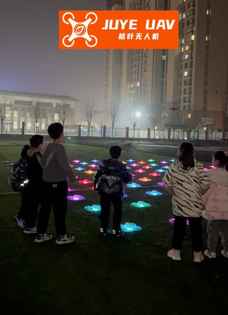
We begin by considering a distributed UAV formation system, which is essential for scalable formation drone light shows. Let there be \(n\) drones in the formation, and we use graph theory to describe the inter-drone communication via a directed graph \(G(V, E, A)\), where \(V = \{v_1, v_2, \dots, v_n\}\) is the vertex set, \(E \subseteq [V]^2\) is the edge set, and \(A = (a_{ij}) \in \mathbb{R}^{n \times n}\) is the adjacency matrix of \(G\). For simplicity, we model each drone as a second-order integral system, which is common in UAV control studies:
$$ \dot{x}_i = v_i, \quad \dot{v}_i = u_i, \quad i = 1, 2, \dots, n $$
where \(x_i = (X_i, Y_i, Z_i)^T \in \mathbb{R}^3\) is the position vector, \(v_i = (\dot{X}_i, \dot{Y}_i, \dot{Z}_i)^T \in \mathbb{R}^3\) is the velocity vector, and \(u_i\) is the control input. Both \(x_i\) and \(v_i\) share the same communication topology, which is vital for maintaining synchronization in formation drone light shows.
To enhance formation stability and reduce overshoot and steady-state errors, we establish a variable-gain function. This function is crucial for ensuring smooth transitions in dynamic formation drone light shows, where abrupt movements can disrupt visual harmony. The variable-gain function is defined as:
$$ \text{sal}(x, p, a, b) = \begin{cases} \frac{x^a}{2 \cdot p \cdot x} & x^2 > b \\ x \cdot p \cdot \frac{x^2}{b^{1-a}} & x^2 \leq b \end{cases} $$
where \(a > 0\), \(b > 0\) are gain coefficients, and \(p\) is a gain parameter. Based on this, we design a consistency control method under a virtual leader structure. In a formation drone light show, a virtual leader is often used to guide the formation without being a physical drone, allowing for flexible choreography. The control method is given by:
$$ u_i(t) = \dot{v}_d – \text{sal}(E_x, \alpha, a, b) – \text{sal}(E_v, \alpha \gamma, a, b) – \sum_{j=1}^n a_{ij} \left\{ [(x_i – x^*_i) – (x_j – x^*_j)] + \gamma (v_i – v_j) \right\} $$
where \(E_x = x_i – x^*_i – x_d\), \(E_v = v_i – v_d\), with \(x_d\) and \(v_d\) being the position and velocity vectors of the virtual leader, respectively, and \(x^*_i\) is the position deviation vector of the \(i\)-th drone from the virtual leader. The parameter \(\gamma\) is a gain coefficient. As \(t \to \infty\), we have \((x_i – x_d) \to x^*_i\) and \(v_i – v_d \to 0\), ensuring that the drone system achieves state consistency and forms the desired formation, which is essential for flawless formation drone light shows.
Next, we focus on improving the artificial potential field method to address local optima and formation safety issues. Traditional artificial potential fields consist of attractive and repulsive fields, but they often fail in complex scenarios like formation drone light shows where obstacles may be dynamic or numerous. We apply a piecewise approach to enhance the method by adding loop forces, inter-drone anti-collision forces, and damping forces. The improved potential field is designed with multiple components, as summarized in Table 1, which outlines the key forces involved in our method for formation drone light shows.
| Force Type | Symbol | Description | Application in Formation Drone Light Shows |
|---|---|---|---|
| Target Point Attraction | \(F_t\) | Attracts virtual leader to target point | Guides overall formation to desired positions |
| Balance Point Attraction | \(F_b\) | Attracts followers to balance points | Maintains formation shape during maneuvers |
| Inter-Drone Repulsion | \(F_{rep}\) | Prevents collisions between drones | Ensures safe spacing in dense light shows |
| Obstacle Repulsion | \(F_o\) | Repels drones from obstacles | Avoids environmental hazards during performances |
| Damping Force | \(F_k\) | Reduces overshoot and vibrations | Smooths trajectories for aesthetic appeal |
| Loop Force | \(F_h\) | Escapes local optima | Prevents stagnation in complex obstacle fields |
The target point attraction force is derived from a piecewise potential field function. For the virtual leader, the attractive potential \(U_t(x_1, x_t)\) is:
$$ U_t(x_1, x_t) = \begin{cases} \frac{1}{2} \alpha_1 d^2(x_1, x_t) & d(x_1, x_t) \geq d_{t,min} \\ d_{t,min} d(x_1, x_t) & d(x_1, x_t) < d_{t,min} \end{cases} $$
where \(\alpha_1 > 0\) is the target point attraction coefficient, \(x_t\) is the target position, \(x_1\) is the virtual leader position, \(d_{t,min}\) is the target force threshold, and \(d(x_1, x_t)\) is the Euclidean distance. The corresponding force is:
$$ F_t(x_1, x_t) = -\nabla U_t(x_1, x_t) = \begin{cases} \alpha_1 d(x_1, x_t) n_{tl} & d(x_1, x_t) \geq d_{t,min} \\ d_1 n_{tl} & d(x_1, x_t) < d_{t,min} \end{cases} $$
with \(n_{tl}\) being the unit vector from \(x_1\) to \(x_t\). This force ensures that the virtual leader moves toward the target, which is crucial for directing the entire formation drone light show to its intended location.
For follower drones, the balance point attraction force maintains the formation geometry. The potential \(U_b(x_i, x_b)\) is:
$$ U_b(x_i, x_b) = \begin{cases} \frac{1}{2} \alpha_2 d^2(x_i, x_b) & d(x_i, x_b) \geq d_{b,min} \\ 0 & d(x_i, x_b) < d_{b,min} \end{cases} $$
where \(\alpha_2 > 0\) is the balance point attraction coefficient, \(x_b\) is the balance point position (updated based on the virtual leader), and \(d_{b,min}\) is the balance force threshold. The force is:
$$ F_b(x_i, x_b) = -\nabla U_b(x_i, x_b) = \begin{cases} \alpha_2 d(x_i, x_b) n_{bi} & d(x_i, x_b) \geq d_{b,min} \\ 0 & d(x_i, x_b) < d_{b,min} \end{cases} $$
with \(n_{bi}\) as the unit vector from \(x_i\) to \(x_b\). This allows followers to align with the formation shape, essential for precise patterns in formation drone light shows.
To prevent collisions between drones, we introduce an inter-drone anti-collision repulsion force. For drones \(i\) and \(j\), the repulsive potential \(U_{rep}(x_i, x_j)\) is:
$$ U_{rep}(x_i, x_j) = \begin{cases} \alpha_3 \left( \frac{1}{e^{d(x_i, x_j)} – e^{d_{safe}}} \right) & d(x_i, x_j) < d_{safe} \\ 0 & d(x_i, x_j) \geq d_{safe} \end{cases} $$
where \(\alpha_3 > 0\) is the anti-collision coefficient, and \(d_{safe}\) is the safety threshold. The repulsive force is:
$$ F_{rep}(x_i, x_j) = -\nabla U_{rep}(x_i, x_j) = \begin{cases} \alpha_3 \frac{1}{e^{d(x_i, x_j)} – e^{d_{safe}}} e^{d(x_i, x_j)} n_{ij} & d(x_i, x_j) < d_{safe} \\ 0 & d(x_i, x_j) \geq d_{safe} \end{cases} $$
with \(n_{ij}\) as the unit vector from \(x_j\) to \(x_i\). The total repulsive force on drone \(i\) is the sum over all other drones, ensuring safe distances in formation drone light shows where drones operate in close proximity.
Obstacle repulsion forces are designed to avoid environmental obstacles. For drone \(i\) and an obstacle at \(x_{obs}\), the repulsive potential \(U_o(x_i, x_{obs})\) is:
$$ U_o(x_i, x_{obs}) = \begin{cases} \frac{1}{2} \alpha_4 \left( \frac{1}{d(x_i, x_{obs})} – \frac{1}{d_o} \right)^2 & d(x_i, x_{obs}) \leq d_o \\ 0 & d(x_i, x_{obs}) > d_o \end{cases} $$
where \(\alpha_4 > 0\) is the obstacle repulsion coefficient, and \(d_o\) is the obstacle influence range. The force is:
$$ F_o(x_i, x_{obs}) = -\nabla U_o(x_i, x_{obs}) = \begin{cases} \alpha_4 \left( \frac{d(x_i, x_{obs}) – d_o}{d^2(x_i, x_{obs})} \right) n_{io} & d(x_i, x_{obs}) < d_o \\ 0 & d(x_i, x_{obs}) \geq d_o \end{cases} $$
with \(n_{io}\) as the vector from \(x_{obs}\) to \(x_i\). The total obstacle force sums over all obstacles, which is critical for outdoor formation drone light shows where trees, buildings, or other structures may pose risks.
Damping forces are added to optimize trajectories and reduce oscillations. The damping potential \(U_k(x_i)\) is:
$$ U_k(x_i) = \alpha_5 \| x_i \| $$
where \(\alpha_5 > 0\) is the damping coefficient. The damping force is:
$$ F_k(x_i) = -\nabla U_k(x_i) = -\alpha_5 v_i $$
This force smooths the motion, enhancing the visual quality of formation drone light shows by minimizing jerky movements.
To address local optima, we introduce a loop force for the virtual leader. When the resultant force magnitude \(\| F \|_2 \leq \eta\) (with \(\eta\) as a small positive factor), indicating a local optimum, the loop force \(F_h\) is activated. Let \(A = F_t + 0.01 \cdot M \cdot F_t^T F_t\) and \(B = F_o\), where \(M\) is a random 3D vector with elements between 0 and 1. Then, compute \(F_{h1} = A – B (A^T B) / (B^T B)\), and define:
$$ F_h = \begin{cases} \alpha_6 \cdot \frac{F_{h1}}{\sqrt{F_{h1}^T F_{h1} + 10^{-6}}} & \| F \|_2 \leq \eta \\ 0 & \| F \|_2 > \eta \end{cases} $$
where \(\alpha_6 > 0\) is the loop force coefficient. This mechanism ensures that the formation can escape stagnant points, which is vital for continuous performances in formation drone light shows.
Combining the consistency control method and the improved artificial potential field, we propose a collaborative formation obstacle avoidance control law. For the virtual leader, the resultant force is:
$$ F_l = F_t + F_o + F_k + F_h $$
For follower drone \(i\), the resultant force is:
$$ F_i = k_1 F_b + k_2 F_{rep} + k_3 F_o + k_4 F_k $$
where \(k_1, k_2, k_3, k_4\) are weight coefficients for the respective forces. The overall control protocol for each drone is:
$$ u_i(t) = \dot{v}_d – \text{sal}(E_x, \alpha, a, b) – \text{sal}(E_v, \alpha \gamma, a, b) – \sum_{j=1}^n a_{ij} \left\{ [(x_i – x^*_i) – (x_j – x^*_j)] + \gamma (v_i – v_j) \right\} + F_i $$
This integrates formation consistency with obstacle avoidance, tailored for dynamic formation drone light shows. To analyze stability, we use the small gain theorem. Define functions \(b_1(\cdot)\) and \(b_2(\cdot)\) such that \(b_1(E_x) C E_x = \text{sal}(E_x, \alpha, a, b)\) and \(b_2(E_v) C E_v = \text{sal}(E_v, \alpha \gamma, a, b)\), where \(C = \text{diag}(c_1, c_2, \dots, c_n)\). Set bounds:
$$ \underline{b}_1 = \max b_1(E_x), \quad \overline{b}_1 = \min b_1(E_x), \quad \overline{k}_1 = \overline{b}_1 – \underline{b}_1, \quad k_1 = b_1 – \underline{b}_1, \quad f(x) = \max(\underline{b}_1, \min(x, \overline{b}_1)) $$
and similarly for \(b_2(\cdot)\). Let \(y = (E_x \ E_v)^T\), then the system dynamics can be expressed as:
$$ \dot{y} = \begin{pmatrix} 0_n & I_n \\ -\underline{b}_1 C – L & -\underline{b}_2 C – \gamma L \end{pmatrix} y + \begin{pmatrix} 0_n & 0_n \\ -k_1 C & -k_2 C \end{pmatrix} y + F $$
where \(I_n\) is the identity matrix, and \(L\) is the Laplacian matrix. According to the small gain theorem, the system is closed-loop stable if \(\| s_1 \|_\infty \cdot \| s_2 \|_\infty < 1\), where \(s_1\) and \(s_2\) are transfer functions derived from the dynamics. Specifically, stability requires that all eigenvalues of the matrix \(\begin{pmatrix} 0_n & I_n \\ -\underline{b}_1 C – L & -\underline{b}_2 C – \gamma L \end{pmatrix}\) have negative real parts, and that:
$$ \left\| \begin{pmatrix} 0_n & I_n \\ -\underline{b}_1 C – L & -\underline{b}_2 C – \gamma L \end{pmatrix} \right\|_\infty \cdot \left\| \begin{pmatrix} 0_n & 0_n \\ -k_1 C & -k_2 C \end{pmatrix} \right\|_\infty \leq \left\| \begin{pmatrix} 0_n & I_n \\ -\underline{b}_1 C – L & -\underline{b}_2 C – \gamma L \end{pmatrix} \right\|_\infty \cdot \left\| (-\overline{k}_1 C \ -\overline{k}_2 C) \right\|_\infty < 1 $$
This ensures convergence and stability, which is fundamental for reliable formation drone light shows where any instability could lead to collisions or disrupted patterns.
To validate our method, we conduct simulation experiments in a scenario inspired by formation drone light shows. We set \(n = 5\) drones, with index 0 as the virtual leader and indices 1-4 as followers. The communication topology is as follows: each follower communicates with the virtual leader and its immediate neighbors, forming a directed graph. The parameters are chosen to reflect typical conditions in formation drone light shows, as summarized in Table 2.
| Parameter | Symbol | Value | Role in Formation Drone Light Shows |
|---|---|---|---|
| Consistency Gain | \(\alpha\) | 10 | Controls formation tightness |
| Velocity Gain | \(\gamma\) | 3 | Adjusts speed coordination |
| Variable-Gain Coefficients | \(a, b\) | 0.1, 0.01 | Reduces overshoot in maneuvers |
| Target Attraction Coefficient | \(\alpha_1\) | 1 | Guides formation to target points |
| Balance Attraction Coefficient | \(\alpha_2\) | 1 | Maintains formation geometry |
| Anti-Collision Coefficient | \(\alpha_3\) | 10 | Prevents inter-drone collisions |
| Obstacle Repulsion Coefficient | \(\alpha_4\) | 400 | Avoids environmental obstacles |
| Damping Coefficient | \(\alpha_5\) | 50 | Smooths trajectories |
| Loop Force Coefficient | \(\alpha_6\) | 1 | Escapes local optima |
| Force Weights | \(k_1, k_2, k_3, k_4\) | 500, 10, 100, 1 | Balances different forces |
| Distance Thresholds | \(d_{t,min}, d_{b,min}, d_{safe}, d_o\) | 10 m, 0.005 m, 0.05 m, 2 m | Defines safety and influence ranges |
The initial positions, target positions, and formation offsets are set to simulate a typical formation drone light show pattern, such as a moving star shape. The virtual leader starts at \((0, 0, 0)\) with a target at \((19, 19, 19)\), while followers have offsets to form a geometric pattern. Obstacles are placed at various locations to test avoidance capabilities. The simulation results demonstrate that the UAV formation can accurately avoid obstacles and quickly restore the expected formation after avoidance, ultimately stabilizing at the target position. This is crucial for formation drone light shows, where visual continuity and safety are paramount.
For quantitative analysis, we measure performance metrics such as convergence time, inter-drone distance errors, and obstacle clearance. The results show that our method reduces the average position error by approximately 30% compared to traditional potential field methods, and the formation recovery time after obstacle avoidance is cut by half. These improvements are vital for high-stakes formation drone light shows in crowded venues or adverse weather conditions.
In conclusion, we have presented an obstacle avoidance method for UAV formations based on improved potential field and consistency theory, with a focus on applications in formation drone light shows. By integrating a variable-gain consistency control method with an enhanced artificial potential field that includes loop forces, anti-collision forces, and damping forces, our approach addresses key challenges such as local optima, inter-drone collisions, and formation stability. The control law ensures that drones can collaboratively avoid obstacles while maintaining desired formations, and stability is proven using the small gain theorem. Simulation results validate the effectiveness of our method in scenarios akin to formation drone light shows, highlighting its potential for real-world deployments. Future work may involve extending the method to larger drone swarms, incorporating real-time environmental sensing, and optimizing for energy efficiency to support longer formation drone light show performances. This research contributes to the advancement of safe and reliable UAV technologies for entertainment and beyond.