
The rapid proliferation and increasing sophistication of unmanned aerial vehicles (UAVs) have fundamentally altered the modern battlespace. These systems present asymmetric threats that challenge traditional air defense paradigms. Consequently, constructing an effective and resilient anti-UAV combat system has become a paramount military objective. A critical challenge in developing such a system lies in quantifying the value of individual equipment within the complex network of interdependent assets. This paper addresses the lack of effective capability evaluation methods for weapons and equipment within the current anti-UAV combat system. We propose a novel methodology for assessing the system contribution rate of equipment based on Combat Loop Theory. Our approach abstracts the intricate relationships between multi-functional equipment into a network of rings, nodes, and edges. We introduce a fuzzy comprehensive evaluation method to calculate edge weights, deriving a Composite Influence Index to evaluate the system’s overall anti-UAV combat capability. Finally, a contribution rate evaluation model is employed to quantify the specific contribution of each equipment unit to the entire anti-UAV architecture.
1. Modeling the Anti-UAV Combat System
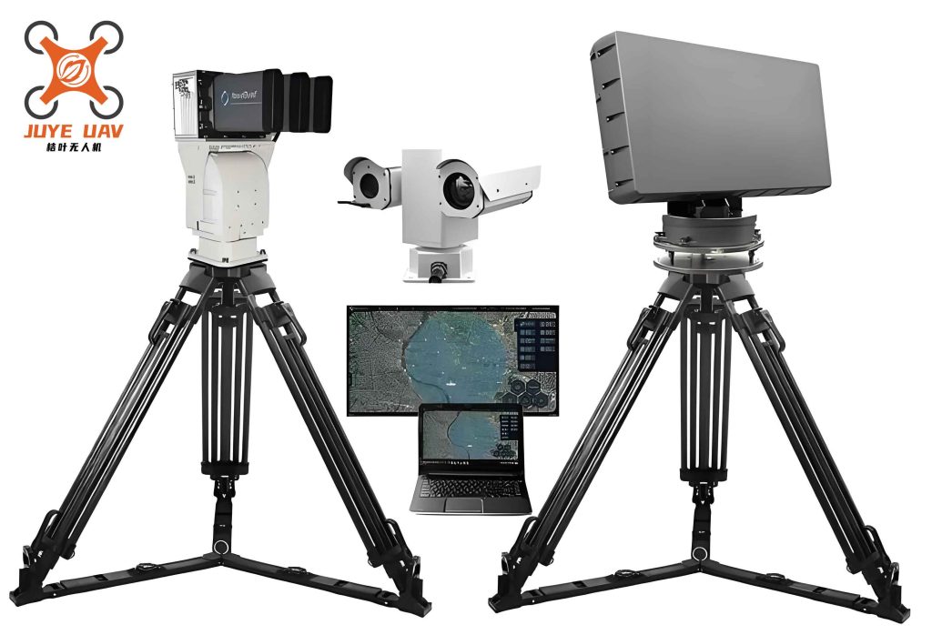
An effective anti-UAV system integrates diverse assets for detection, command and control (C2), and kinetic or non-kinetic effects. A typical system may include low-altitude surveillance radars, electro-optical/infrared sensors, command centers, early warning aircraft, short-range air defense missiles, electronic jammers, and directed-energy weapons. The operational process inherently follows the Observe, Orient, Decide, Act (OODA) loop, which can be abstracted into the concept of a Combat Loop. A Combat Loop is a closed circuit formed by a sequence of nodes representing detection of a target (Observe), information fusion and decision-making (Orient/Decide), execution of an action (Act), and the effect on the target itself.
In our model, we categorize all equipment based on its primary function within an anti-UAV engagement, creating four node types:
- Surveillance Node (S): Equipment with detection and surveillance capabilities (e.g., radars, EO/IR systems).
- Decision Node (D): Equipment with command, control, and information processing capabilities (e.g., command centers, data fusion systems).
- Action Node (A): Equipment with “hard-kill” or “soft-kill” effects (e.g., interceptor missiles, jammers, high-power microwaves).
- Target Node (T): The adversarial UAVs being engaged.
A single physical platform may host multiple functions, thus appearing as different nodes in our functional network. For instance, an integrated air defense system may act as both an S-node (via its organic radar) and a D-node. The directed connections between these functional nodes form the edges (E) of our combat network, representing the flow of information or action (e.g., S→D for reporting, D→A for firing orders, A→T for engagement). The weight of an edge (ω) signifies the probability or effectiveness of that specific connection or interaction.
The construction of the anti-UAV combat network model involves three key steps, as formalized below:
- Define the Mission: Identify the anti-UAV operational objective(s).
- Abstract the System: Based on the objective, define the set of functional nodes U = {S, D, A, T} from available equipment. Establish the set of directed edges E based on potential operational interactions. Determine the weight set ω for these edges.
- Build the Topology: Formally construct the network graph G = (U, E, ω).
The resulting model is a heterogeneous network where the successful engagement of a target UAV is represented by the existence of at least one complete, closed Combat Loop from T (the UAV) back to T via S, D, and A nodes. The strength and number of these loops determine the system’s overall effectiveness against that target.
2. Assessing System Capability via Combat Loops
The core capability of an anti-UAV system is its aggregate ability to negatively affect hostile UAV targets. We measure this using a Composite Influence Index (hG). This index is a weighted sum of the system’s influence on each target type.
Let $T = {T_1, T_2, …, T_m}$ be the set of target UAV types. Let $w_{T_i}$ be the strategic weight or priority of target $T_i$, where $\sum_{i=1}^{m} w_{T_i} = 1$. Let $Ef_{T_i}$ be the total influence capability of the anti-UAV system on target $T_i$. The Composite Influence Index for the entire system network G is calculated as:
$$h_G = \sum_{i=1}^{m} (w_{T_i} \cdot Ef_{T_i})$$
The influence on a specific target, $Ef_{T_i}$, is derived from all Combat Loops that terminate on that target. If $OL_1, OL_2, …, OL_n$ are the n distinct Combat Loops affecting target $T_i$, then:
$$Ef_{T_i} = \sum_{j=1}^{n} U_{OL_j}$$
where $U_{OL_j}$ is the Influence Capability Metric of the j-th Combat Loop.
The metric for a single Combat Loop is defined as the product of the connection probabilities (weights) of all edges constituting that loop. This reflects the likelihood or effectiveness of the entire chain of events. For a loop $OL_j$ consisting of edges $e_1, e_2, …, e_k$, its metric is:
$$U_{OL_j} = \prod_{q=1}^{k} p_{e_q}$$
where $p_{e_q} \in (0, 1]$ is the weight of edge $e_q$.
2.1 Calculating Edge Weights with Fuzzy Comprehensive Evaluation
Determining the edge weights ($p_{e_q}$) is critical. Given the complexity and uncertainty inherent in combat operations, we employ a Fuzzy Comprehensive Evaluation (FCE) method. This translates expert judgment and equipment performance parameters into quantitative connection probabilities.
The FCE process for a given edge (e.g., from a Surveillance node S to a Decision node D) involves five steps:
- Define the Factor Set (X): Identify the key capability indicators influencing the edge’s effectiveness. These are derived from node capability hierarchies for surveillance, decision, or action functions. For an S→D edge, relevant factors may include detection probability ($x_1$), data accuracy ($x_2$), and communication reliability ($x_3$). Thus, $X = {x_1, x_2, x_3}$.
- Define the Evaluation Set (V): Establish qualitative assessment levels. We use four levels: $V = ${Fully Satisfactory (FS), Satisfactory (S), Barely Satisfactory (BS), Unsatisfactory (U)}$. We assign a quantitative score vector: $Y = [1.0, 0.66, 0.33, 0.0]$ corresponding to V.
- Determine Factor Weights (A): Use the Analytic Hierarchy Process (AHP) to determine the relative importance of each factor in X for the specific edge’s function. This yields a weight vector $A = [a_1, a_2, a_3]$, where $\sum a_i = 1$.
- Construct the Fuzzy Evaluation Matrix (R): A panel of experts evaluates the performance of the link for each factor against the evaluation set V. The results are compiled into a matrix R, where element $r_{ij}$ is the membership degree of factor $i$ to evaluation level $j$.
- Perform Comprehensive Evaluation: The fuzzy comprehensive evaluation vector B is obtained by: $B = A \circ R$. The final quantitative weight $p_{edge}$ for the edge is then computed as: $p_{edge} = B \cdot Y^T$.
This process is repeated for all edges in the combat network, populating the weight set ω with values between 0 and 1.
3. Evaluating Equipment Contribution Rate
The system contribution rate of a specific piece of equipment is intuitively understood as the degree to which the overall system’s capability degrades if that equipment is removed or neutralized. Formally, we define the contribution rate $con_{v_i}$ for equipment (or functional node) $v_i$ as:
$$con_{v_i} = \frac{h_G – h_{G-v_i}}{h_G} \times 100\%$$
where:
- $h_G$ is the Composite Influence Index of the original, intact anti-UAV system network.
- $h_{G-v_i}$ is the Composite Influence Index of the degraded network after removing node $v_i$ (and all edges connected to it).
A higher $con_{v_i}$ indicates that the equipment is more critical to the anti-UAV system’s overall effectiveness. This metric allows for a direct comparison of the value of different assets within the networked force structure.
4. Case Study: A Typical Anti-UAV Engagement Scenario
To demonstrate our methodology, we apply it to a notional anti-UAV defense scenario. The Blue force operates large UAVs ($T_1$) and swarms of small UAVs ($T_2$). The Red force deploys a layered defense system comprising the following equipment, abstracted into functional nodes:
| Node ID | Node Type | Representative Equipment |
|---|---|---|
| S1 | Surveillance (S) | Low-Altitude Search Radar |
| S2 | Surveillance (S) | Electro-Optical Radar |
| S3 | Surveillance (S) | IR/EO Detection System |
| S4, D1 | Surveillance (S), Decision (D) | Integrated Air Defense C2 Center |
| S5, D2 | Surveillance (S), Decision (D) | Airborne Early Warning & Control Aircraft |
| S6, D3, A1 | Surv. (S), Dec. (D), Action (A) | Short-Range Air Defense Missile System |
| A2 | Action (A) | Navigation Signal Jammer |
| A3 | Action (A) | High-Power Microwave Interceptor |
| T1 | Target (T) | Large UAV |
| T2 | Target (T) | Small/Medium UAV |
Using the FCE method described, the weights for the primary edge types in this network are calculated. A subset of results is shown below:
| Edge Function | Example Edges | Calculated Weight (p) |
|---|---|---|
| Surveillance-to-Target | T1→S1, T2→S2 | 0.7605 |
| Surveillance-to-Decision | S1→D1, S5→D2 | 0.8563 |
| Decision-to-Action | D1→A2, D3→A1 | 0.8563 |
| Action-to-Target (Kinetic) | A1→T1 | 0.7324 |
| Action-to-Target (Jamming) | A2→T2 | 0.8243 |
| Decision-to-Decision | D2→D1 | 0.8491 |
With the network fully defined and weighted, we identify all distinct Combat Loops. For example, one loop engaging $T_1$ is: $T1 \rightarrow S1 \rightarrow D1 \rightarrow A1 \rightarrow T1$. Its Influence Capability Metric is:
$$U_{OL_{T1-1}} = p_{T1S1} \cdot p_{S1D1} \cdot p_{D1A1} \cdot p_{A1T1} = 0.7605 \times 0.8563 \times 0.8563 \times 0.7324 \approx 0.4084$$
We calculate this for all loops. Assume the analysis yields 12 effective loops against $T_1$ and 10 against $T_2$. The summed influences are:
$$Ef_{T1} = \sum_{j=1}^{12} U_{OL_{T1-j}} = 4.5212, \quad Ef_{T2} = \sum_{j=1}^{10} U_{OL_{T2-j}} = 4.1038$$
Assigning strategic weights $w_{T1}=0.7$ and $w_{T2}=0.3$, the system’s Composite Influence Index is:
$$h_G = (0.7 \times 4.5212) + (0.3 \times 4.1038) = 4.3960$$
4.1 Contribution Rate Analysis
We now compute the contribution rate for each key equipment node by removing it from the network and recalculating $h_{G-v_i}$. For instance, removing the Short-Range Air Defense Missile System (which provides nodes S6, D3, A1) results in a new index $h_{G-A1} = 2.8566$. Its contribution rate to the anti-UAV system is:
$$con_{A1} = \frac{4.3960 – 2.8566}{4.3960} \times 100\% \approx 35.02\%$$
Performing this calculation for all major nodes yields the following contribution rates:
| Equipment / Functional Node | System Contribution Rate (%) |
|---|---|
| Low-Altitude Search Radar (S1) | 35.72 |
| Electro-Optical Radar (S2) | 24.52 |
| IR/EO Detection System (S3) | 8.41 |
| Integrated Air Defense C2 Center (S4, D1) | 97.21 |
| Airborne Early Warning (S5, D2) | 16.66 |
| Short-Range Air Defense System (S6, D3, A1) | 35.02 |
| Navigation Signal Jammer (A2) | 36.28 |
| High-Power Microwave Interceptor (A3) | 28.71 |
5. Discussion and Implications
The results from our case study offer valuable insights for anti-UAV system design and resource allocation. The extremely high contribution rate (97.21%) of the Integrated Air Defense C2 Center (S4, D1) underscores the critical, central role of command, control, and data fusion in a networked anti-UAV architecture. It acts as a key hub, and its loss would cripple most engagement loops. This highlights the need for robust protection, redundancy, and resilience for such C2 nodes in any anti-UAV system.
The high contribution of soft-kill systems like the Navigation Signal Jammer (A2 at 36.28%) validates the importance of electronic warfare capabilities in countering UAV threats, often providing a cost-effective and scalable solution, especially against swarms.
Furthermore, the analysis reveals a strong correlation between a node’s contribution rate and its betweenness centrality—the number of Combat Loops in which it participates. Nodes that form part of many alternative paths to engage targets are naturally more valuable to the overall anti-UAV network’s robustness. The model also confirms that shorter Combat Loops (with fewer edges) generally have higher Influence Capability Metrics ($U_{OL}$), indicating that faster, more direct engagement chains are preferable for reliability and effectiveness.
Our methodology, based on Combat Loop theory and fuzzy evaluation, provides a structured, quantitative framework for assessing equipment within an anti-UAV system. It moves beyond evaluating platforms in isolation and instead measures their value within the interdependent network required for modern counter-drone operations. This approach can inform critical decisions throughout the lifecycle of anti-UAV capabilities, from research and development prioritization and acquisition to operational deployment and force structuring. By identifying the most critical nodes (high $con_{v_i}$), commanders can focus protective measures and develop contingency plans, while planners can identify potential single points of failure and work to create more resilient, redundant anti-UAV architectures.