
The proliferation of unmanned aerial vehicles (UAVs), or drones, across military domains presents a persistent and evolving threat. Their small size, low radar cross-section, low-altitude flight profiles, and potential for swarming tactics challenge traditional air defense systems based on kinetic interceptors. In this context, directed energy weapons, particularly high-energy laser (HEL) systems, have emerged as a promising countermeasure. Shipborne laser weapons offer a deep magazine, low cost-per-shot, speed-of-light engagement, and scalable effects—from sensor dazzling to physical destruction. This paper focuses on the combat effectiveness evaluation of a representative ten-kilowatt class shipborne laser system for the anti-drone mission. We develop a comprehensive, module-based simulation framework to model the end-to-end engagement chain, from beam propagation through the maritime atmosphere to target damage assessment, providing a theoretical basis for estimating optimal intercept ranges and kill probabilities against a typical tactical UAV.
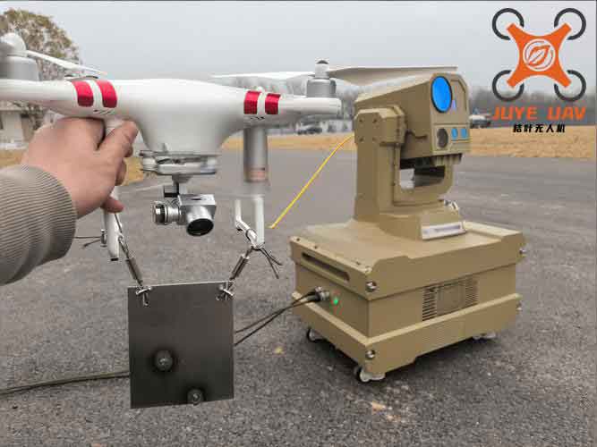
The core advantage of a laser-based anti-drone system lies in its engagement physics. Unlike missiles, a laser weapon delivers energy at the speed of light, effectively negating the need for lead-angle prediction against maneuvering targets. The destructive mechanism is thermal, relying on depositing sufficient energy density on a vulnerable part of the target to cause functional degradation (soft-kill) or structural failure (hard-kill). The effectiveness is governed by a fundamental inequality: the delivered fluence (energy per unit area) must exceed the target’s damage threshold fluence for a given irradiation time. This is expressed as:
$$E_{delivered} = \int_{0}^{T} I(t) \, dt \geq E_{threshold}(P_{threshold}, T)$$
where \(I(t)\) is the irradiance (power density, W/cm²) on target at time \(t\), \(T\) is the total irradiation time, and \(E_{threshold}\) is the required energy density (J/cm²) which is a function of a critical power density \(P_{threshold}\) and time. For a constant irradiance, this simplifies to \(I \cdot T \geq E_{threshold}\). The challenge in a realistic anti-drone scenario is that \(I(t)\) is not constant; it is severely degraded by range, atmospheric conditions, and pointing inaccuracies.
Target Characterization and Vulnerability Modeling
Effective anti-drone analysis begins with a clear understanding of the threat. We select a representative target: a ship-based vertical take-off and landing (VTOL) tactical UAV, analogous to systems like the MQ-8C. Key parameters for such a target are summarized below.
| Parameter | Value / Description |
|---|---|
| Type | VTOL Tactical UAV (e.g., for reconnaissance, targeting) |
| Max Speed | ~260 km/h |
| Cruise Speed | ~230 km/h |
| Operational Altitude | Up to 6,000 m |
| Critical Components | EO/IR sensor turret, composite skin, fuel cells, control surfaces |
For modeling purposes, the complex geometry of the drone is simplified. A critical component, such as the electro-optical/infrared (EO/IR) sensor dome for a soft-kill or a section of the composite skin over a fuel cell for a hard-kill, is represented as a target circle of effective radius \(r_{t}\). The drone’s flight path is modeled as linear motion with a possible dive angle \(\theta_m\). Its position in a Cartesian coordinate system (with the laser weapon at the origin) at time step \(i\) is given by:
$$
\begin{aligned}
x(i) &= x_0 – V_m \cos(\theta_m) \cdot t_i \\
y(i) &= y_0 + V_m \sin(\theta_m) \cdot t_i \quad \text{(Altitude)} \\
z(i) &= z_0 \quad \text{(Cross-range)}
\end{aligned}
$$
The instantaneous slant range \(R\) to the target and the laser’s required line-of-sight angles (elevation \(\epsilon\), azimuth \(\beta\)) are then:
$$
R = \sqrt{x(i)^2 + y(i)^2 + z(i)^2}, \quad \epsilon = \arctan\left(\frac{y(i)}{\sqrt{x(i)^2 + z(i)^2}}\right), \quad \beta = \arctan\left(\frac{z(i)}{x(i)}\right)
$$
The vulnerability of the drone is defined by material damage thresholds. Composite materials like glass-fiber/epoxy or carbon-fiber/epoxy used in skins and structures have distinct ablation thresholds. Sensitive optics in EO/IR systems are vulnerable to much lower irradiance levels. We define two primary anti-drone kill mechanisms:
| Kill Mechanism | Target Component | Typical Threshold Irradiance (Pth) | Required Fluence (Eth) |
|---|---|---|---|
| Soft-Kill (Dazzle/Disable) | EO/IR Sensor Dome | ~70 W/cm² | ~700 J/cm² (for 10s dwell) |
| Hard-Kill (Destruction) | Composite Skin / Fuel Cell | ~300 W/cm² | ~1500 J/cm² (for 5s dwell) |
Atmospheric Propagation: The Primary Limiting Factor
The maritime atmosphere is the most significant factor degrading laser performance in a shipborne anti-drone role. Two main effects must be quantified: attenuation (reduction of beam power) and turbulence (degradation of beam quality and aiming stability).
1. Atmospheric Attenuation: Laser power is attenuated along the path by molecular absorption and aerosol (haze, mist, sea spray) scattering. The transmittance \(T\) over a path length \(R\) is modeled by the Beer-Lambert law. For horizontal paths, a common empirical model relates transmittance to visibility \(V\):
$$T_{horizontal} = \exp\left( -\frac{3.912}{V} \cdot \left(\frac{\lambda}{0.55 \mu m}\right)^{-q} \cdot R \right)$$
where \(\lambda\) is the laser wavelength (e.g., 1.064 μm for a Nd:YAG laser), and \(q\) is a coefficient dependent on visibility (\(q \approx 1.3\) for 6 km < V < 20 km). For slant paths to an aerial target, a more complex model accounting for the atmospheric profile is used. The power reaching the target plane, \(P_r\), is:
$$P_r = P_0 \cdot T$$
where \(P_0\) is the laser’s exit power.
2. Atmospheric Turbulence: Temperature and pressure variations cause refractive index fluctuations (\(C_n^2\)), known as optical turbulence. This leads to beam wander (motion of the centroid), beam spreading (beyond the diffraction limit), and scintillation (intensity fluctuations). The key parameter describing turbulence-induced beam spread is the atmospheric coherence width or Fried parameter, \(r_0\). For a spherical wave (a good approximation for a propagated beam), it is given by:
$$r_0 = \left[ 0.423 \cdot k^2 \cdot \int_{0}^{R} C_n^2(h(s)) \, ds \right]^{-3/5}$$
where \(k = 2\pi/\lambda\) is the wave number. The refractive index structure constant \(C_n^2(h)\) varies with altitude \(h\). A standard model for the maritime boundary layer is the Hufnagel-Valley (HV) model. The turbulence-induced beam quality factor \(\beta_t\) is related to the ratio of the transmitter aperture diameter \(D\) to \(r_0\):
$$\beta_t \approx \sqrt{1 + 2.99 \left(\frac{D}{r_0}\right)^{5/3}}$$
The overall beam quality factor \(\beta\) after propagating through turbulence, combining the laser’s intrinsic beam quality \(\beta_0\) and the turbulence effect, is approximately:
$$\beta \approx \sqrt{\beta_0^2 + \beta_t^2}$$
This degraded beam quality directly increases the beam’s spot size on the distant target, reducing irradiance.
Beam Projection, Spot Size, and Tracking Accuracy
The irradiance on target is critically dependent on the area over which the delivered power \(P_r\) is distributed. The diffraction-limited beam spot radius (containing ~84% of the energy for a uniform circular beam) at range \(R\) is:
$$w_{dl} = \frac{1.22 \cdot \lambda \cdot R}{D}$$
Accounting for the degraded beam quality \(\beta\), the actual spot radius \(w\) becomes:
$$w = \beta \cdot w_{dl} = \frac{1.22 \cdot \beta \cdot \lambda \cdot R}{D}$$
The geometric area of this spot on a surface normal to the beam is \(A_{spot} = \pi w^2\). However, in an anti-drone engagement, the target surface is often at an oblique angle \(\phi\) to the beam. The projected spot area on the target surface is larger: \(A_{proj} \approx A_{spot} / |\cos \phi|\). Furthermore, the beam does not hold perfectly steady on the aimpoint. Tracking system errors (jitter) and atmospheric tilt (beam wander) cause the beam centroid to randomly move around the desired aimpoint. This pointing error, typically modeled as a zero-mean Gaussian distribution with standard deviation \(\sigma_{pe}\) (in radians), is a crucial factor. The effective irradiance on the small target area is determined by the overlap between the intensity profile of the wobbly beam and the target area.
We model this using a Monte Carlo approach. For each simulation time step, a random pointing offset \((\theta_x, \theta_y)\) is drawn from the distribution \(\mathcal{N}(0, \sigma_{pe})\). This offset deflects the beam center on the target plane. The distance \(d\) between the beam center and the target center is calculated. The total power deposited on the target is the integral of the beam intensity profile \(I_{beam}(r)\) over the target area. For a top-hat beam profile approximation and a circular target of radius \(r_t\), the overlap area \(A_{overlap}\) can be calculated geometrically:
$$
A_{overlap} =
\begin{cases}
\pi r_t^2, & \text{if } d \leq w – r_t \quad \text{(target inside beam)} \\
\text{Intersection Formula}, & \text{if } |w – r_t| < d < w + r_t \\
0, & \text{if } d \geq w + r_t \quad \text{(complete miss)}
\end{cases}
$$
The average irradiance on the target for that time step is then:
$$I_{avg}(t) = \frac{P_r \cdot \left( \frac{A_{overlap}(t)}{\pi w^2} \right) \cdot \alpha}{A_{target}}$$
where \(\alpha\) is the target surface absorptivity at the laser wavelength, and \(A_{target} = \pi r_t^2\). The fraction in parentheses represents the power fraction hitting the target. The cumulative fluence (energy density) delivered is the time integral of \(I_{avg}(t)\).
Integrated Combat Effectiveness Simulation Model
We integrate the aforementioned modules into a sequential simulation framework to assess the anti-drone effectiveness of a 10-kW class laser. The system parameters and simulation constants are defined as follows:
| Laser System Parameter | Symbol | Value |
|---|---|---|
| Output Power | \(P_0\) | 10 kW / 30 kW / 100 kW (for comparison) |
| Wavelength | \(\lambda\) | 1.064 μm |
| Transmitter Aperture Diameter | \(D\) | 0.3 m |
| Initial Beam Quality | \(\beta_0\) | 3 |
| Tracking/Pointing Error (1σ) | \(\sigma_{pe}\) | 10 μrad |
| Engagement & Environment Parameter | Symbol | Value / Range |
|---|---|---|
| Maritime Visibility | \(V\) | 15 km, 25 km, 40 km |
| Target Diving Angle | \(\theta_m\) | 0° (level), 5° (diving) |
| Target Absorptivity | \(\alpha\) | 0.8 |
| Target Effective Radius (Sensor) | \(r_t\) | 0.1 m |
The simulation loop for a single engagement run proceeds as follows:
1. Initialize: Set target initial conditions \((x_0, y_0, z_0, V_m, \theta_m)\), laser parameters, and atmospheric conditions (\(V\), \(C_n^2\) profile).
2. Time Step Update: Calculate target position, range \(R\), and line-of-sight angles.
3. Atmospheric Effects: Calculate path transmittance \(T(R, V)\) and turbulence-degraded beam quality \(\beta(R, C_n^2)\).
4. Beam-Target Geometry: Calculate beam spot size \(w(R, \beta)\), generate random pointing error, and compute overlap area \(A_{overlap}\).
5. Target Irradiance & Fluence: Compute \(I_{avg}(t)\) and update cumulative fluence \(E_{cumulative} = \int I_{avg}(t) dt\).
6. Kill Assessment: Check if \(I_{avg}(t) \geq P_{th}\) and \(E_{cumulative} \geq E_{th}\) for the desired kill mechanism.
7. Loop: Repeat steps 2-6 until the target passes by or kill conditions are met.
8. Monte Carlo Iteration: Repeat the entire engagement run (e.g., 1000 times) with different random pointing error seeds to generate statistical results.
The primary output is the Probability of Kill (PK) as a function of engagement range or initial conditions. The effective intercept range is defined as the maximum range at which PK remains above a required threshold (e.g., 0.9 or 0.99).
Simulation Results and Analysis for Anti-Drone Engagements
Running the integrated model provides quantitative insights into the capabilities and limitations of a 10-kW class laser in the anti-drone role. The results are highly sensitive to atmospheric visibility.
Scenario 1: Soft-Kill against EO/IR Sensor (Pth=70 W/cm², Eth=700 J/cm²). Target in a shallow dive (5°), initial altitude 3000 m, initial slant range 5000 m.
| Atmospheric Visibility (V) | Effective Intercept Range (PK ≥ 0.99) | Key Limiting Factor |
|---|---|---|
| 15 km | ~4.4 km | Attenuation reduces on-target power; larger spot size from turbulence reduces irradiance. |
| 25 km | ~4.9 km | Reduced attenuation allows slightly longer engagement range. |
Scenario 2: Hard-Kill against Structure (Pth=300 W/cm², Eth=1500 J/cm²). Target in a shallow dive, initial altitude 2000 m, initial slant range 2500 m.
| Atmospheric Visibility (V) | Effective Intercept Range (PK ≥ 0.99) | Key Limiting Factor |
|---|---|---|
| 15 km | ~1.7 km | Very high threshold fluence demands high irradiance, limiting range severely even in moderate haze. |
| 25 km | ~2.0 km | Improved visibility extends the hard-kill envelope marginally. |
The relationship between visibility and maximum engagement range is strongly non-linear, particularly for hard-kill. The performance cliff is evident. To overcome atmospheric limitations, increasing laser power is the most direct countermeasure. For instance, scaling the laser power to 100 kW significantly extends the effective anti-drone range. For a soft-kill mission against a sensor, the effective range in 25 km visibility can extend beyond 7 km, while a hard-kill range may reach 3-4 km under the same conditions. This highlights the critical trade-off in laser weapon design: power scaling is essential for robust performance against hardened drone components at tactically useful ranges.
The simulation also reveals the profound impact of tracking accuracy. The 10 μrad error budget, while good, still causes significant power to spill off the small target area at longer ranges. The anti-drone effectiveness curve (PK vs. Range) typically shows a rapid drop-off rather than a gentle decline, emphasizing the “keeper’s zone” concept where the laser must maintain precise aim on a vulnerable spot for a sustained period to achieve kill.
Conclusion
This paper has presented a detailed, physics-based modeling and simulation framework for evaluating the combat effectiveness of shipborne high-energy laser weapons in the anti-drone mission. By integrating models for target dynamics, maritime atmospheric propagation (attenuation and turbulence), beam projection, tracking inaccuracies, and target vulnerability, we can quantify the key performance metric: Probability of Kill as a function of engagement range.
The analysis confirms that a ten-kilowatt class laser is a viable system for countering tactical drones, particularly for soft-kill missions (sensor dazzling) at ranges of several kilometers in fair weather. However, achieving hard-kill against structural components is much more challenging, requiring shorter engagement distances due to the higher irradiance and fluence thresholds. Atmospheric visibility is the dominant environmental factor determining effective range. Beam quality degradation from turbulence and tracking system jitter are secondary but critical factors that dilute the on-target power density.
The framework clearly demonstrates that increasing laser power is the primary lever for extending robust anti-drone capabilities, especially for hard-kill and operations in degraded meteorological conditions. Future work will involve refining the models with higher-fidelity data, incorporating dynamic target maneuvers and swarming behaviors, and analyzing the integration of laser weapons with other kinetic and electronic anti-drone systems in a layered ship defense architecture. This modeling approach provides essential theoretical underpinnings for the development, requirements specification, and tactical deployment of directed energy weapons for naval force protection against the growing drone threat.