
The rapid growth of mobile data traffic and the demand for ubiquitous connectivity have motivated the research community to explore new communication paradigms beyond the fifth generation (5G) system. Two promising technologies for the sixth generation (6G) system are unmanned aerial vehicle (UAV) communications and extremely large-scale multiple-input multiple-output (XL-MIMO) systems. The unmanned aerial vehicle (UAV) brings flexibility, fast deployment, and strong line-of-sight (LoS) links, while XL-MIMO offers extremely high spectral efficiency and spatial resolution through a very large number of antennas. However, as the antenna aperture increases, the Rayleigh distance becomes very large, and the UAV is likely to operate in the near-field region of the XL-MIMO array. Therefore, conventional far-field assumptions are no longer valid, and new design approaches are needed.
In this article, we present our research on UAV position optimization and wireless transmission methods based on XL-MIMO. We first consider a downlink communication scenario where a UAV equipped with an XL uniform planar array (UPA) serves multiple single-antenna users. By using spherical-wave channel modeling, we derive a set of near-field orthogonal positions for users. Then we propose user scheduling and UAV altitude optimization algorithms to maximize the achievable sum rate. In the second part, we study the beam tracking problem for a high-mobility UAV served by a ground XL-MIMO base station. We combine the state evolution model and the extended Kalman filter (EKF) to predict the UAV motion range, and design a wide beamforming vector based on the near-field codebook to minimize the variance of the beam gain over the coverage range. Simulation results show that the proposed methods significantly improve the system performance and reliability.
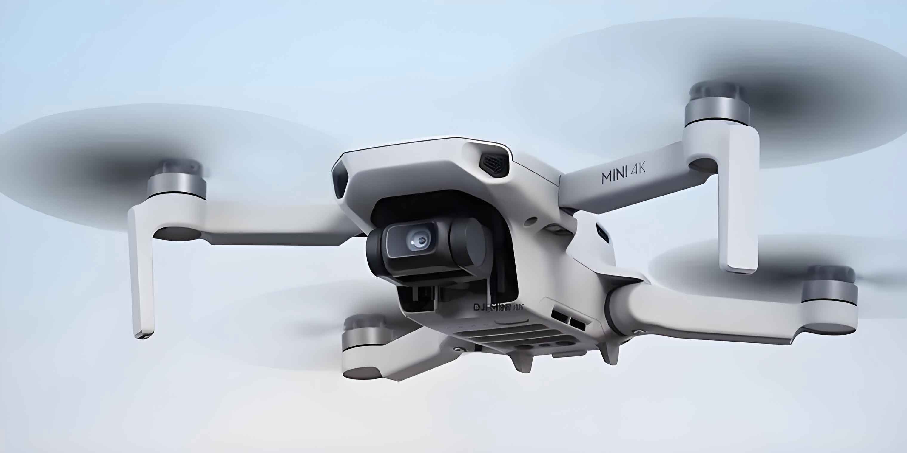
1. Introduction
The fifth generation mobile communication system has been deployed worldwide, but the growing demand for higher data rates, wider coverage, and massive connectivity has led to extensive research on the sixth generation (6G) system. In 6G, the coverage will extend to space, air, ground, and sea, forming an integrated network. The unmanned aerial vehicle (UAV) is a key component of such an integrated network because it can be flexibly deployed as an aerial base station, relay, or mobile edge computing node. The UAV-assisted communication system can provide LoS links, which significantly reduces path loss and improves reliability. Moreover, large antenna arrays can be mounted on UAVs to support high-gain beamforming. However, UAVs have limited size and energy, so efficient position optimization and transmission schemes are required.
XL-MIMO systems are characterized by an extremely large number of antennas, typically hundreds or thousands, which can be deployed in linear, planar, or cylindrical configurations. The large aperture of XL-MIMO arrays leads to a much larger Rayleigh distance compared with conventional massive MIMO systems. In the near-field region, the wavefront is spherical rather than planar, so the array response depends on both angle and distance. This new degree of freedom can be exploited to distinguish users in the spatial domain, but it also makes channel modeling and beamforming design more challenging. Existing studies on UAV position optimization mostly focus on the far-field region. With the increasing number of antennas, the near-field effect cannot be ignored. Therefore, it is necessary to investigate UAV position optimization and beam tracking methods under near-field XL-MIMO channels.
In this article, we make the following contributions:
- We derive a set of near-field orthogonal positions for users in a UAV-assisted XL-MIMO downlink system. When users are located at these positions, their channel vectors are mutually orthogonal, thereby eliminating inter-user interference.
- We propose a user scheduling algorithm and a UAV altitude optimization algorithm based on the derived orthogonal positions. The user scheduling algorithm selects users and assigns them to the orthogonal positions to minimize interference and movement distance, and the altitude optimization algorithm uses particle swarm optimization (PSO) to find the optimal UAV altitude.
- We propose a near-field beam tracking method for a high-mobility UAV. The method uses the EKF to predict the UAV position and determines the beam coverage range in the angle and distance domains. A wide beamforming vector is designed based on the near-field codebook, and its phase parameters are optimized to minimize the variance of the beam gain within the coverage.
2. System Model of UAV-Enabled XL-MIMO Downlink Transmission
We consider a downlink communication system where a UAV acts as an aerial base station and serves \(K\) single-antenna users. The UAV is equipped with an XL uniform planar array comprising \(M_x \times M_y\) antennas, and the total number of antennas is \(M = M_x M_y\). The array lies in the \(xOy\) plane, and the first antenna is placed at the origin. The antenna spacing is \(d\), and the carrier wavelength is \(\lambda\). The \(m\)-th antenna is located at \(\mathbf{q}_m = [i_m d, j_m d, 0]^T\), where \(i_m \in \{0,1,\dots,M_x-1\}\) and \(j_m \in \{0,1,\dots,M_y-1\}\). The user \(k\) is located at \(\mathbf{q}_k = [x_k, y_k, H]^T\), where \(H\) is the UAV altitude. Its spherical coordinates are \((r_k, \theta_k, \phi_k)\), where \(r_k = \sqrt{x_k^2 + y_k^2 + H^2}\), \(\theta_k = \arccos(H/r_k)\), and \(\phi_k = \arctan(y_k/x_k)\).
Because the UAV is usually much higher than the surrounding scatterers, the LoS component dominates the air-to-ground channel, and the NLoS component can be neglected. Therefore, the channel vector between the UAV and user \(k\) is written as
$$ \mathbf{h}_k = \frac{\lambda}{4\pi r_k} e^{-j\frac{2\pi}{\lambda} r_k} \mathbf{a}(\theta_k,\phi_k,r_k), $$
where \(\mathbf{a}(\theta_k,\phi_k,r_k)\) is the near-field spherical-wave array response vector. The \(m\)-th element of this vector is given by
$$ [\mathbf{a}(\theta_k,\phi_k,r_k)]_m = \frac{1}{\sqrt{M}} e^{-j\frac{2\pi}{\lambda}(r_k^{(m)} – r_k)}, $$
and \(r_k^{(m)}\) is the distance from the \(m\)-th antenna to user \(k\), expressed as
$$ r_k^{(m)} = \sqrt{r_k^2 + (i_m d)^2 + (j_m d)^2 – 2 r_k d\left(i_m \sin\theta_k \cos\phi_k + j_m \sin\theta_k \sin\phi_k\right)}. $$
The received signal vector at the \(K\) users is
$$ \mathbf{y} = \sqrt{\frac{P}{K}} \mathbf{H} \mathbf{W} \mathbf{s} + \mathbf{n}, $$
where \(P\) is the total transmit power, \(\mathbf{H} = [\mathbf{h}_1, \mathbf{h}_2, \cdots, \mathbf{h}_K]^H\) is the channel matrix, \(\mathbf{W} = [\mathbf{w}_1, \mathbf{w}_2, \cdots, \mathbf{w}_K]\) is the beamforming matrix, \(\mathbf{s}\) is the data vector with \(\mathbb{E}[\mathbf{s}\mathbf{s}^H] = \mathbf{I}_K\), and \(\mathbf{n} \sim \mathcal{CN}(0, \sigma^2 \mathbf{I}_K)\) is the noise vector. We adopt matched-filter (MF) beamforming, i.e., \(\mathbf{w}_k = \mathbf{h}_k / \|\mathbf{h}_k\|\). Then the achievable sum rate is given by
$$ R = \frac{1}{K}\sum_{k=1}^{K} \log_2\left(1 + \frac{\frac{\rho}{K} |\mathbf{h}_k^H \mathbf{w}_k|^2}{1 + \frac{\rho}{K} \sum_{j\neq k} |\mathbf{h}_k^H \mathbf{w}_j|^2}\right), $$
where \(\rho = P/\sigma^2\) is the transmit signal-to-noise ratio (SNR). The objective is to maximize \(R\) by jointly optimizing the user positions and the UAV altitude. The optimization problem is
$$ \max_{\{x_k,y_k\}, H} R \quad \text{s.t.} \quad k \in \{1,2,\dots,K\}, \quad H_{\min} \le H \le H_{\max}. $$
This problem is non-convex and difficult to solve directly. Therefore, we first derive a set of orthogonal positions that make the user channels mutually orthogonal, and then we design efficient scheduling and altitude optimization algorithms.
3. Near-Field Orthogonal Positions and Optimization Algorithms
3.1 Derivation of Orthogonal Positions
The inter-user interference in the sum-rate expression mainly depends on the inner product \(\mathbf{h}_p^H \mathbf{h}_q\). If we can find positions such that the channel vectors of different users are orthogonal, the interference can be completely eliminated. Based on the spherical-wave channel model, we derive the following theorem.
Theorem 1: Consider an XL-UPA with \(M_x \times M_y\) antennas and carrier wavelength \(\lambda\). The near-field orthogonal positions can be organized into \(S\) layers, and each layer contains \(N\) angular positions. Let \(\mathbf{p}_n^{(s)} = [r_{s,n}, \theta_n, \phi_n]^T\) denote the \(n\)-th orthogonal position on the \(s\)-th layer. Then the azimuth angle \(\phi_n\), elevation angle \(\theta_n\), and radial distance \(r_{s,n}\) are given by
$$ \phi_n = \arctan\left(\frac{2m_y-1}{2m_x-1}\cdot\frac{M_y}{M_x}\right), $$
$$ \theta_n = \arcsin\left(\frac{\lambda}{d}\sqrt{\left(\frac{2m_x-1}{M_x}\right)^2 + \left(\frac{2m_y-1}{M_y}\right)^2}\right), $$
$$ r_{s,n} = \frac{Z_x}{s\left(1-2\sin^2\theta_n\cos^2\phi_n\right)}, $$
or equivalently
$$ r_{s,n} = \frac{Z_y}{s\left(1-2\sin^2\theta_n\sin^2\phi_n\right)}, $$
where \(Z_x\) and \(Z_y\) are constants determined by the array geometry and a preset threshold, \(m_x \in \mathcal{M}_x\), \(m_y \in \mathcal{M}_y\), \(n\in\{1,2,\dots,N\}\), and \(s\in\{1,2,\dots,S\}\). The values of \(m_x\) and \(m_y\) are selected to ensure that \(\sin\theta_n\in[0,1]\).
The theorem shows that the orthogonal positions are not only separated in angle but also in distance. This is a fundamental difference from the far-field case, where only angular separation is required. In the near-field regime, the distance dimension provides an additional degree of freedom for spatial multiplexing. This property is particularly useful for UAV communication systems, because the UAV altitude and the user locations jointly determine the distance and angle distributions.
In our scenario, the users are located on the sea surface, so their vertical coordinates are approximately zero. Since the orthogonal positions are discrete points in three-dimensional space, we need to select those positions that lie on the sea surface. We define a tolerance \(\Delta_H\) to account for wave fluctuations. If the vertical coordinate of a generated orthogonal position falls in the interval \([H-\Delta_H, H+\Delta_H]\), it is considered as a sea-surface orthogonal position. The resulting set of sea-surface positions is denoted as \(\mathcal{P} = \{\mathbf{p}_1,\mathbf{p}_2,\dots,\mathbf{p}_L\}\), where \(L\) is the number of available positions for a given altitude \(H\).
3.2 User Scheduling Algorithm
For a fixed UAV altitude \(H\), the number of sea-surface orthogonal positions \(L\) may be smaller than the number of users \(K\). In that case, only \(L\) users can be moved to the orthogonal positions, and the remaining users stay at their initial positions. The scheduling problem is therefore to select the most suitable users and assign them to the orthogonal positions. We formulate a binary assignment problem with variables \(b_{k,l}\), where \(b_{k,l}=1\) if user \(k\) is assigned to position \(l\), and \(b_{k,l}=0\) otherwise. The constraints are
$$ \sum_{l=1}^{L} b_{k,l} \le 1, \quad \forall k, $$
$$ \sum_{k=1}^{K} b_{k,l} \le 1, \quad \forall l. $$
If \(K \le L\), the Hungarian algorithm can be directly applied to minimize the total movement distance. If \(K > L\), we first select \(L\) users who suffer the strongest interference from other users. To this end, we compute an interference metric for each user based on the cross-channel inner products:
$$ r_{k,l}^{(i)} = \sum_{\substack{k’=1 \\ k’ \neq k}}^{K} \frac{|\mathbf{h}_{k’}^H \mathbf{h}_k|}{\|\mathbf{h}_{k’}\| \|\mathbf{h}_k\|}, $$
and we select the \(L\) users with the largest metrics. Then the Hungarian algorithm is used to assign these selected users to the orthogonal positions with minimum total movement distance. This user scheduling algorithm is called the interference-channel-interference-based selection (ICIBS) algorithm, and it is summarized in Algorithm 1. We use “Algorithm 1” as a logical block in our implementation, but the details can be easily programmed in MATLAB.
| Step | Operation |
|---|---|
| 1 | Input: altitude \(H\), orthogonal position set \(\mathcal{P}\), user set \(\mathcal{K}\). |
| 2 | If \(K > L\), compute the interference metric for every user. |
| 3 | Select \(L\) users with the largest interference metric. |
| 4 | Use the Hungarian algorithm to assign the selected users to \(\mathcal{P}\). |
| 5 | If \(K \le L\), use the Hungarian algorithm for all users. |
| 6 | Output: the assignment variable \(b_{k,l}\) for all \(k,l\). |
3.3 UAV Altitude Optimization Algorithm
The number of sea-surface orthogonal positions changes with the UAV altitude, because the distance layers and the angle coverage vary with \(H\). Therefore, the user scheduling result also depends on \(H\). To maximize the sum rate, we optimize the UAV altitude using particle swarm optimization (PSO). In each iteration, for each particle representing a candidate altitude, we first generate the sea-surface orthogonal positions, then apply the user scheduling algorithm, and finally compute the sum rate. The PSO algorithm updates the particle velocities and positions according to
$$ \mathbf{v}^{(t)} = w\mathbf{v}^{(t-1)} + c_1 r_1\left(\mathbf{U}_{\mathrm{best}}^{(t-1)} – \mathbf{U}^{(t-1)}\right) + c_2 r_2\left(\mathbf{U}_{\mathrm{global}} – \mathbf{U}^{(t-1)}\right), $$
$$ \mathbf{U}^{(t)} = \mathbf{U}^{(t-1)} + \mathbf{v}^{(t)}, $$
where \(w\) is the inertia weight, \(c_1\) and \(c_2\) are acceleration coefficients, \(r_1\) and \(r_2\) are random numbers uniformly distributed in \([0,1]\), \(\mathbf{U}_{\mathrm{best}}\) is the personal best position, and \(\mathbf{U}_{\mathrm{global}}\) is the global best position. The altitude is bounded by \(H_{\min}\) and \(H_{\max}\). The PSO-based altitude optimization algorithm is summarized in Algorithm 2.
| Step | Operation |
|---|---|
| 1 | Initialize \(Q\) particles with random altitudes and zero velocities. |
| 2 | For each particle, generate the sea-surface orthogonal positions for the given altitude. |
| 3 | Run Algorithm 1 to obtain the user assignment and compute the sum rate. |
| 4 | Update personal best and global best based on the sum rate. |
| 5 | Update velocities and altitudes using the PSO update equations. |
| 6 | Repeat until the maximum number of iterations is reached. |
| 7 | Output the optimal altitude \(H_{\mathrm{opt}}\) and the corresponding user assignment. |
3.4 Simulation Results for the First System
We conducted simulations to evaluate the proposed near-field orthogonal position design and optimization algorithms. The simulation parameters are listed in Table 1. The users are randomly distributed in a 200 m \(\times\) 300 m rectangular area.
| Parameter | Value |
|---|---|
| Number of antennas \(M_x, M_y\) | 250, 20 |
| Number of users \(K\) | 120 |
| Carrier frequency \(f\) | 30 GHz |
| Antenna spacing \(d\) | 0.005 m |
| Threshold parameter \(\beta_\Delta\) | 1.2 |
| UAV altitude range | [10 m, 200 m] |
Figure 3.2 in our study illustrates the initial user positions and the optimized positions when the UAV altitude is 100 m and \(K=25\). The sea-surface orthogonal positions are 20 for this altitude. Since the number of users is larger than the number of orthogonal positions, only 20 users can be moved to the orthogonal positions, while the remaining 5 users stay at their initial positions. This demonstrates the effectiveness of the proposed scheduling algorithm.
The relationship between the number of orthogonal positions and the UAV altitude is shown in Figure 3.3. We observe that the number of orthogonal positions first increases and then decreases with the altitude. This is because the spatial resolution and the distance-domain layers vary with the distance between the UAV and the users. The sum rate follows a similar trend, which indicates that the proposed orthogonal positions significantly affect the system performance. Therefore, optimizing the UAV altitude is crucial.
In Figure 3.4, we compare the proposed scheme with three baselines: (1) users remain at their initial positions and only the altitude is optimized, (2) the Hungarian algorithm is used without the ICIBS selection, and (3) a discrete search algorithm for altitude optimization. The proposed scheme achieves the highest sum rate over the whole SNR range. The performance gain comes from the fact that users are placed at the near-field orthogonal positions, which greatly reduces the inter-user interference. When the number of users is smaller than the number of orthogonal positions, the proposed algorithm reduces to the Hungarian algorithm. When the number of users is larger, the ICIBS selection provides additional performance improvement by moving the users with the most severe interference.
4. Beam Tracking for a High-Mobility UAV in XL-MIMO Near-Field
In the second part, we consider a different scenario where a ground base station equipped with an XL-UPA serves a single-antenna UAV. The UAV moves at high speed and always remains within the near-field region of the base station. Because the beam generated by the XL-MIMO array is very narrow, the UAV may quickly move out of the beam coverage, resulting in severe performance degradation. Therefore, we propose a beam tracking method that uses the predicted UAV position and a wide beam design to maintain reliable communication.
4.1 System Model and Problem Formulation
The base station is equipped with \(M_x \times M_y\) antennas, and the antenna spacing is \(d = \lambda/2\). The position of the UAV at time \(t\) is denoted as \(\mathbf{p}(t) = [r(t), \theta(t), \phi(t)]^T\) in spherical coordinates. The channel vector is
$$ \mathbf{h}(t) = \frac{\lambda}{4\pi r(t)} e^{-j\frac{2\pi}{\lambda}r(t)} \mathbf{a}(\theta(t),\phi(t),r(t)), $$
where the near-field array response is defined similarly to (3.4). The received signal is
$$ y(t) = \sqrt{P} \mathbf{h}^H(t)\mathbf{f}(t) s(t) + n(t), $$
where \(\mathbf{f}(t)\) is the beamforming vector with \(\|\mathbf{f}(t)\|=1\). The beam gain at the UAV position is
$$ \gamma(\mathbf{p}(t)) = \left|\mathbf{a}^H(\theta(t),\phi(t),r(t)) \mathbf{f}(t)\right|^2. $$
Since the UAV moves during a frame, the channel is not constant within each frame. To avoid beam misalignment, we design a beamforming vector whose main lobe covers the entire UAV motion range in the current frame. The objective is to minimize the variance of the beam gain over the coverage range. Thus, the optimization problem is
$$ \min_{\mathbf{f}} \quad \mathrm{Var}\left\{\gamma(\mathbf{p}_u)\right\}, \quad \text{s.t.} \quad \mathbf{p}_u \in \mathcal{B}, \quad \|\mathbf{f}\|=1, $$
where \(\mathcal{B}\) denotes the beam coverage range and \(\mathbf{p}_u\) are uniformly sampled points inside \(\mathcal{B}\).
4.2 UAV Position Acquisition via Extended Kalman Filter
We model the UAV state as \(\mathbf{c}(t) = [\mathbf{p}^T(t), \mathbf{v}^T(t)]^T\), where \(\mathbf{v}(t)\) is the velocity vector. The state evolution equation is
$$ \mathbf{c}(t_k) = \mathbf{A}\mathbf{c}(t_{k-1}) + \mathbf{n}_c(t_k), $$
with the state transition matrix
$$ \mathbf{A} = \begin{bmatrix} \mathbf{I}_3 & T_f \mathbf{I}_3 \\ \mathbf{0}_3 & \mathbf{I}_3 \end{bmatrix}, $$
where \(T_f\) is the frame duration. The processing noise \(\mathbf{n}_c(t_k)\) has covariance matrix \(\mathbf{Q}\). In addition, the base station observes the phase differences of the received signal across the antennas. The measurement equation is
$$ \mathbf{z}(t_k) = \mathbf{g}(\mathbf{p}(t_k)) + \mathbf{n}_p(t_k), $$
where \(\mathbf{g}(\cdot)\) is the phase-difference measurement function and \(\mathbf{n}_p(t_k)\) is the measurement noise with covariance matrix \(\mathbf{R}_p\). Since the measurement function is nonlinear, we use the extended Kalman filter (EKF) to estimate the UAV state. The EKF prediction and update equations are
$$ \mathbf{m}_{k|k-1} = \mathbf{A}\mathbf{m}_{k-1|k-1}, $$
$$ \mathbf{P}_{k|k-1} = \mathbf{A}\mathbf{P}_{k-1|k-1}\mathbf{A}^T + \mathbf{Q}, $$
$$ \mathbf{K}_k = \mathbf{P}_{k|k-1}\mathbf{G}_k^T\left(\mathbf{G}_k\mathbf{P}_{k|k-1}\mathbf{G}_k^T + \mathbf{R}_p\right)^{-1}, $$
$$ \mathbf{m}_{k|k} = \mathbf{m}_{k|k-1} + \mathbf{K}_k(\mathbf{z}(t_k) – \mathbf{g}(\mathbf{m}_{k|k-1})), $$
$$ \mathbf{P}_{k|k} = \left(\mathbf{I} – \mathbf{K}_k\mathbf{G}_k\right)\mathbf{P}_{k|k-1}, $$
where \(\mathbf{G}_k\) is the Jacobian matrix of \(\mathbf{g}\) evaluated at the predicted state. The EKF provides an accurate estimate of the UAV position at the current frame and also predicts the position for the next frame.
4.3 Beam Coverage Determination
Based on the estimated position at the current frame \(\mathbf{p}^-\) and the predicted position at the next frame \(\mathbf{p}^+\), we determine the beam coverage range in the angular and distance domains. Using the \(3\sigma\) principle, the elevation angle coverage is
$$ \Theta = [\theta_c – 3\sigma_\theta^-,\ \theta_c + 3\sigma_\theta^+], $$
where \(\theta_c = (\theta^- + \theta^+)/2\) is the center elevation angle, and \(\sigma_\theta^-\) and \(\sigma_\theta^+\) are the standard deviations of the estimated and predicted elevation angles, respectively. Similarly, the azimuth angle coverage is
$$ \Phi = [\phi_c – 3\sigma_\phi^-,\ \phi_c + 3\sigma_\phi^+]. $$
For the radial distance, the near-field codebook divides the space into discrete layers. For a given estimated position, we find the layer index \(s^-\) such that the distance \(r^-\) lies between two adjacent layers, and we find the layer index \(s^+\) for the predicted position \(r^+\). The distance coverage includes all layers from \(\min(s^-,s^+)\) to \(\max(s^-,s^+)+1\). The selected quantization points inside the beam coverage are then used to construct the beamforming vector.
4.4 Beamforming Design with Phase Optimization
Let \(\{\theta_l,\phi_l,r_l\}_{l=1}^{L}\) be the set of quantization points selected from the near-field codebook inside the coverage range. We design the beamforming vector as a superposition of the near-field array responses corresponding to these quantization points:
$$ \mathbf{f} = \frac{1}{\sqrt{L}}\sum_{l=1}^{L} e^{j\eta_l} \mathbf{a}(\theta_l,\phi_l,r_l), $$
where \(\eta_l\) is the phase parameter of the \(l\)-th component. Unlike the far-field gradient-phase design, the phase parameters here are individually optimized because the near-field phase is nonlinear. The optimization problem is
$$ \min_{\eta_1,\dots,\eta_L} \mathrm{Var}\left\{\gamma(\mathbf{p}_u)\right\}, \quad \text{s.t.} \quad \eta_l \in [0,2\pi], \quad l=1,\dots,L, $$
where \(\mathbf{p}_u\) are uniformly sampled points in the beam coverage. We use PSO to solve this non-convex problem. The algorithm updates the phase parameters according to the same velocity and position update rules as in the previous section. The resulting beamforming vector has a relatively flat gain over the coverage range, which ensures stable reception quality while the UAV is moving.
| Parameter | Value |
|---|---|
| Number of antennas \(M_x, M_y\) | 250, 50 |
| Carrier frequency \(f\) | 30 GHz |
| Transmit SNR \(\rho\) | 100 dB |
| Number of frames \(K\) | 10 |
| Number of slots per frame \(\Gamma\) | 10 |
| Frame duration \(T_f\) | 1 s |
| Initial state \(\mathbf{c}(t_0)\) | \([1,0.5,21,0.97,0,1]^T\) |
| Process noise variances | \([0.1^2,0,0.1^2]^T\) |
4.5 Simulation Results for the Second System
We evaluated the proposed beam tracking method in terms of received SNR and average achievable rate. Figure 4.3 in our study shows the true trajectory, the predicted trajectory from the state evolution model, and the EKF-estimated trajectory. The EKF estimate is much closer to the true trajectory than the state evolution prediction. This verifies the effectiveness of the EKF in the near-field XL-MIMO scenario.
We also studied the effect of the number of sampling points \(U\) on the variance of the beam gain. The variance decreases as \(U\) increases, but the improvement becomes marginal when \(U\) is larger than 60. Therefore, we set \(U=60\) in the simulations to balance performance and complexity.
Figure 4.5 compares the proposed beam tracking scheme with two baselines: (1) MF fixed beam pointing to the current frame start position, and (2) a gradient-phase wide beam method. The MF fixed beam suffers from severe SNR fluctuations because the UAV quickly moves out of the narrow beam. The gradient-phase method provides a wider beam but its gain variation is still larger than the proposed method. The proposed scheme maintains a relatively stable received SNR throughout the frames, which demonstrates the advantage of the near-field codebook-based wide beam design with phase optimization.
Figure 4.6 shows the average achievable rate per frame. The proposed method achieves the highest average rate among the three schemes. The MF fixed beam has the lowest rate because of frequent beam misalignment. The gradient-phase method performs better than the MF fixed beam but is still inferior to the proposed method. This indicates that the proposed phase optimization is effective in the near-field region, where the gradient-phase assumption is no longer accurate.
Finally, we verified the convergence of the PSO algorithm used in the beamforming design. Figure 4.7 shows the variance of the beam gain versus the number of iterations for the first, fourth, and eighth frames. In all cases, the variance decreases rapidly and converges within a small number of iterations. This confirms the stability and practicality of the proposed optimization algorithm.
5. Conclusion
In this article, we have studied UAV position optimization and wireless transmission methods for XL-MIMO systems. In the first scenario, we considered a UAV-enabled XL-MIMO downlink system with multiple users. By exploiting the near-field spherical-wave channel, we derived a set of orthogonal user positions and proposed user scheduling and UAV altitude optimization algorithms. The simulation results demonstrated that the proposed orthogonal positions can significantly reduce inter-user interference, and the joint optimization algorithm improves the achievable sum rate compared with the baselines. In the second scenario, we considered a high-mobility UAV served by a ground XL-MIMO base station. We proposed a beam tracking method based on the EKF, near-field codebook quantization, and PSO-based phase optimization. The proposed method maintains a stable received SNR over the UAV motion range and achieves a higher average rate than the existing beamforming methods. These results highlight the importance of taking the near-field effect into account when designing UAV communication systems with XL-MIMO arrays.
For future work, we plan to extend the proposed methods to multi-UAV scenarios and to consider more practical channel models with imperfect position information. In addition, the security and energy efficiency of the near-field UAV communication system are also important topics worth investigating. The combination of unmanned aerial vehicle communication and XL-MIMO near-field transmission will play a key role in the future 6G wireless networks.