
The rapid advancement of artificial intelligence and robotics technologies has significantly expanded the application domains of unmanned aerial vehicles (UAVs), ranging from military reconnaissance to civilian logistics and disaster response. As a core enabling technology for autonomous flight, path planning directly determines the efficiency, safety, and mission success rate of UAV operations in complex environments. In particular, three-dimensional path planning in cluttered and terrain-rich environments poses substantial challenges due to the high-dimensional search space, nonlinear constraints, and the need for real-time responsiveness. This thesis focuses on developing improved path planning methodologies for unmanned aerial vehicles operating in complex three-dimensional environments, addressing the limitations of existing algorithms in terms of convergence accuracy, local optima avoidance, and path executability.
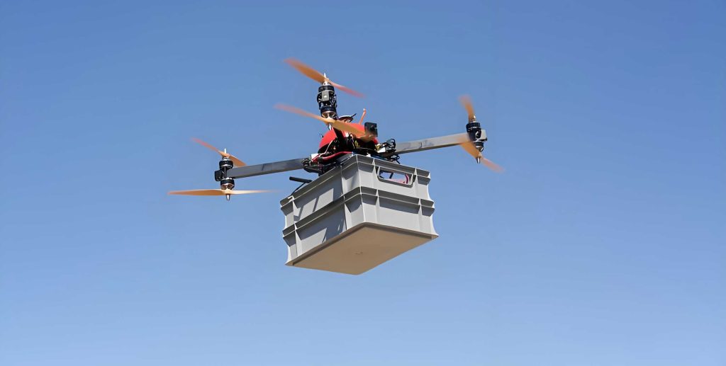
To tackle the challenges above, the thesis makes the following key contributions. First, an Adaptive Hybrid Artificial Bee Particle Swarm Optimization (AHAPSO) algorithm is proposed for UAV path planning in complex terrain environments. Second, a Fusion of Particle Swarm Optimization and Artificial Potential Field (FPAPF) method is developed to address the local minima and unreachable target problems in dense obstacle environments. Third, a comprehensive evaluation framework incorporating path metrics and controller-in-the-loop trajectory tracking is established to validate the executability of planned paths from a control perspective.
Problem Formulation for UAV Path Planning
UAV path planning seeks to find a collision-free path from a start point to a target point while minimizing a cost function that balances multiple objectives. In this thesis, the path is represented by a sequence of n waypoints ${(X\_1, Y\_1, Z\_1), (X\_2, Y\_2, Z\_2), …, (X\_n, Y\_n, Z\_n)}$ within a three-dimensional environment. The total cost function integrates five components: path length, collision risk, flight altitude, path smoothness, and radar threat.
Path Length Cost
The path length cost f₁ accumulates the Euclidean distances between consecutive waypoints, which directly reflects flight efficiency and energy consumption.
$$
f_1 = \sum_{i=1}^{n-1} \sqrt{(X_{i+1} – X_i)^2 + (Y_{i+1} – Y_i)^2 + (Z_{i+1} – Z_i)^2}
\tag{1}
$$
Collision Cost
The collision cost f₂ penalizes path points that are too close to terrain surfaces or obstacles. Let Δdᵢ = zᵢ − zₑ(xᵢ, yᵢ) denote the vertical clearance between the waypoint zᵢ and terrain height zₑ. The collision cost is defined as:
$$
f_2 =
\begin{cases}
+\infty, & \exists i, \Delta d_i \le 0 \\
\sum_{i=1}^{n} \frac{c_{punk}}{\Delta d_i}, & \Delta d_i > 0
\end{cases}
\tag{2}
$$
Flight Altitude Cost
The altitude cost f₃ ensures that the UAV maintains a preferred altitude range to reduce ground proximity risks and radar exposure. With a minimum allowable altitude z_min, maximum z_max, and ideal mean altitude z_mean = (z_min + z_max) ⁄ 2, the cost is:
$$
f_3 = \sum_{i=1}^{n} p_{h,i}, \quad
p_{h,i} =
\begin{cases}
h_{punk} \left( \frac{z_i – z_{mean}}{z_{max} – z_{min}} \right)^{2}, & z_{min} < z_i < z_{max}, \\
100 h_{punk}, & \text{otherwise}.
\end{cases}
\tag{3}
$$
Path Smoothness Cost
Smoothness cost f₄ penalizes sharp turns and abrupt climb angle changes to ensure the path is flyable by fixed-wing aircraft. The cost incorporates turn angle θ_{turn,i} and climb angle φᵢ at each waypoint:
$$
f_4 = \sum_{i=2}^{n-1} \left[ \lambda_{turn} \left( \max(0, |\theta_{turn,i}| – \theta_{max}) \right)^2 + \lambda_{climb} \left( \max(0, |\phi_i – \phi_{i-1}| – \phi_{max}) \right)^2 \right]
\tag{4}
$$
Radar Threat Cost
For mission scenarios with radar threats, the cost f₅ penalizes entering radar detection zones. With radar positions radarⱼ, detection radius rⱼ, safe buffer Δs, and threat coefficient ω_radar:
$$
f_5 = \sum_{i=1}^{n} \sum_{j=1}^{m}
\begin{cases}
+\infty, & d_{i,j} \le r_j, \\
\frac{\omega_{radar}}{d_{i,j} – r_j}, & r_j < d_{i,j} \le r_j + \Delta s, \\
0, & d_{i,j} > r_j + \Delta s.
\end{cases}
\tag{5}
$$
Finally, the weighted total cost function Fit = Σᵢ bᵢfᵢ (i = 1,…,5) is formulated with Σᵢ bᵢ = 1, and serves as the fitness function for the optimization algorithms.
AHAPSO: Adaptive Hybrid Particle Swarm Optimization for 3D Path Planning
Although particle swarm optimization (PSO) has been widely applied to UAV path planning due to its simplicity and global search capability, it suffers from premature convergence and poor exploitation in complex three-dimensional terrains. To overcome these limitations, this thesis proposes AHAPSO, which integrates four complementary enhancement mechanisms into the canonical PSO framework.
Adaptive Inertia Weight
Instead of the traditional linear decreasing inertia weight, AHAPSO adopts a nonlinear exponential adaptation strategy:
$$
\omega = \omega_1 \cdot \exp\left( -\frac{iter}{N} \right)
\tag{6}
$$
where ω₁ is the initial maximum inertia weight, iter is the current iteration number, and N is the total number of iterations. This strategy maintains intensive exploration at the early stage, gradually shifting toward exploitation in later iterations, effectively balancing global exploration and local refinement.
Employed Bee Strategy for Local Search
Inspired by the artificial bee colony (ABC) algorithm, AHAPSO incorporates an employed bee phase to strengthen local search capability around the current promising regions. For each particle i, a new candidate position is generated as:
$$
x_{ij}^{new} = x_{ij} + \phi_{ij}(x_{ij} – x_{kj})
\tag{7}
$$
where k ≠ i is a randomly selected particle index, and φᵢⱼ is a uniform random number in [−1, 1]. This mechanism enriches the neighborhood search diversity and helps refine local solutions.
Mutation Mechanism
To prevent premature convergence and maintain population diversity, a mutation operation is applied to particle velocities with a small probability. The mutated velocity is given by:
$$
v_{mut}^i = \text{rand}(0,1) \cdot (v_{max} – v_{min}) + v_{min}
\tag{8}
$$
Logistic Chaotic Mapping in Late Iterations
In the last 25% of iterations, a Logistic chaotic map is introduced to enhance the algorithm’s ability to escape local optima. The chaotic value c_v is computed as:
$$
c_v = m \times \text{rand} \times (1 – \text{rand})
\tag{9}
$$
Each particle’s position is then adjusted as pₙ = pₛ + cᵥ × (b_max − b_min), where pₛ and pₙ are the pre- and post-mapping positions, and [b_min, b_max] are the boundary constraints. The chaotic traversal property aids in redirecting the search trajectory into unexplored regions.
Algorithm Flow and Complexity
The workflow of AHAPSO proceeds as follows: (1) initializing particles; (2) evaluating fitness values; (3) updating velocity and position with adaptive inertia; (4) applying mutation with small probability; (5) conducting employed bee local search; (6) updating personal and global bests; (7) applying chaotic mapping in the late stage; and (8) outputting the global optimum. Table 1 summarizes the parameters used for AHAPSO and the comparison algorithms.
| Algorithm | Key Parameters |
|---|---|
| PSO | w = 0.8; c₁ = c₂ = 1.5 |
| GWO | a = 2 − 2t/T; A = 2ar₁ − a; C = 2r₂ |
| DBO | P_percent = 0.2; R(t) = 1 − t/M; θ = π/180·k |
| SSA | P% = 0.2; ρ = 0.8; NSD = 20 |
| AHAPSO | w = 0.9·exp(−t/T); c₁ = c₂ = 1.5; pₘ = 0.1; µ = 4 |
The overall time complexity of AHAPSO remains O(NM(P + f)) where N is the maximum iterations, M denotes the swarm size, P is the number of path points per particle, and f represents the computational cost of the fitness function. The mutation and chaotic mechanisms introduce only O(M) additional overhead, preserving the computational attractiveness of PSO.
Numerical Experiments on CEC2017 Benchmark
To validate the effectiveness of AHAPSO, comprehensive experiments were conducted on the CEC2017 benchmark suite comprising 29 test functions with dimensions of 30. The population size and maximum iterations were set to 30 and 1000, respectively. Each algorithm was independently run 30 times to record the best (Best), mean (Mean), and standard deviation (STD) values.
Effectiveness of Individual Improvement Strategies
To analyze the contribution of each mechanism, four AHAPSO variants were constructed by gradually adding strategies: AHAPSO.1 (adaptive inertia only), AHAPSO.2 (+ employed bee), AHAPSO.3 (+ chaotic map), and the full AHAPSO (+ mutation). Table 2 presents the representative results.
| Fun. | PSO | AHAPSO.1 | AHAPSO.2 | AHAPSO.3 | AHAPSO | |||||
|---|---|---|---|---|---|---|---|---|---|---|
| Mean | STD | Mean | STD | Mean | STD | Mean | STD | Mean | STD | |
| F1 | 4.19E+08 | 5.75E+08 | 5.04E+08 | 7.68E+08 | 5.53E+08 | 1.10E+09 | 5.48E+08 | 1.08E+09 | 3.77E+03 | 4.92E+03 |
| F6 | 6.39E+02 | 9.98E+00 | 6.20E+02 | 1.42E+01 | 6.10E+02 | 7.07E+00 | 6.10E+02 | 7.07E+00 | 6.07E+02 | 8.92E+00 |
| F12 | 2.18E+07 | 1.11E+08 | 2.84E+07 | 1.16E+08 | 9.48E+07 | 4.02E+08 | 8.77E+07 | 3.64E+08 | 2.79E+05 | 2.08E+05 |
| F22 | 4.32E+03 | 2.28E+03 | 4.14E+03 | 1.95E+03 | 3.34E+03 | 1.42E+03 | 3.34E+03 | 1.42E+03 | 3.17E+03 | 1.62E+03 |
| F30 | 2.09E+04 | 3.23E+04 | 4.79E+04 | 1.06E+05 | 6.36E+04 | 1.78E+05 | 6.38E+04 | 1.78E+05 | 1.14E+04 | 3.74E+03 |
The results demonstrate that while the adaptive inertia weight alone yields only marginal improvements, the integration of the employed bee phase and chaotic mapping contributes to enhanced search accuracy. The mutation mechanism provides the most significant performance gain, indicating its critical role in maintaining population diversity and escaping local optima. The complete AHAPSO achieves superior mean values on the majority of functions, confirming the complementarity of the proposed mechanisms.
Comparative Performance Evaluation
The proposed AHAPSO was compared against PSO, GWO, DBO, and SSA on the CEC2017 benchmark. Table 3 reports the complete results, where +, =, and − indicate that AHAPSO is better, equal, or worse than the competitor, respectively.
| Fun. | PSO | GWO | DBO | SSA | AHAPSO | ||||||||||
|---|---|---|---|---|---|---|---|---|---|---|---|---|---|---|---|
| Best | Mean | STD | Best | Mean | STD | Best | Mean | STD | Best | Mean | STD | Best | Mean | STD | |
| F1 | 2.15E+06 | 3.88E+07 | 4.42E+07 | 1.25E+02 | 1.23E+09 | 1.34E+09 | 4.62E+08 | 2.26E+09 | 1.26E+09 | 1.08E+02 | 3.00E+03 | 3.25E+03 | 1.35E+02 | 6.31E+03 | 5.97E+03 |
| F4 | 4.92E+02 | 6.50E+02 | 1.34E+02 | 4.73E+02 | 6.59E+02 | 1.20E+02 | 5.03E+02 | 6.14E+02 | 8.11E+01 | 4.64E+02 | 4.97E+02 | 2.98E+01 | 4.25E+02 | 4.79E+02 | 2.41E+01 |
| F6 | 6.34E+02 | 6.46E+02 | 1.12E+01 | 6.02E+02 | 6.10E+02 | 7.56E+00 | 6.21E+02 | 6.46E+02 | 1.23E+01 | 6.23E+02 | 6.45E+02 | 1.21E+01 | 6.01E+02 | 6.08E+02 | 5.39E+00 |
| F9 | 1.23E+03 | 3.58E+03 | 2.55E+03 | 9.13E+02 | 2.61E+03 | 2.02E+03 | 1.17E+03 | 2.33E+03 | 8.82E+02 | 4.21E+03 | 5.30E+03 | 3.42E+02 | 9.02E+02 | 1.62E+03 | 9.10E+02 |
| F16 | 2.85E+03 | 3.20E+03 | 4.21E+02 | 2.15E+03 | 2.60E+03 | 3.46E+02 | 2.00E+03 | 2.53E+03 | 3.30E+02 | 2.31E+03 | 2.92E+03 | 3.43E+02 | 1.87E+03 | 2.44E+03 | 2.84E+02 |
| F22 | 2.56E+03 | 5.12E+03 | 2.01E+03 | 2.30E+03 | 4.10E+03 | 1.76E+03 | 2.43E+03 | 4.73E+03 | 2.07E+03 | 2.30E+03 | 6.73E+03 | 1.44E+03 | 2.30E+03 | 2.92E+03 | 1.32E+03 |
| F26 | 4.61E+03 | 6.46E+03 | 1.40E+03 | 2.90E+03 | 5.05E+03 | 1.06E+03 | 3.67E+03 | 4.85E+03 | 4.89E+02 | 2.90E+03 | 6.28E+03 | 1.58E+03 | 2.80E+03 | 3.62E+03 | 1.00E+03 |
| F30 | 2.78E+05 | 5.33E+06 | 8.38E+06 | 6.33E+03 | 4.52E+04 | 1.06E+05 | 1.35E+06 | 9.91E+06 | 7.21E+06 | 6.49E+03 | 1.30E+04 | 5.22E+03 | 6.08E+03 | 1.05E+04 | 4.00E+03 |
From the Friedman rank test, the average ranks are: AHAPSO (1.17), GWO (2.91), SSA (3.26), DBO (3.43), and PSO (4.22). AHAPSO attains the lowest rank, indicating superior overall performance across diverse function types. The W/T/L statistics (26 wins, 1 tie, 2 losses against SSA; 29 wins against others) demonstrate the robustness and competitiveness of AHAPSO in handling complex optimization landscapes.
3D Path Planning Simulation with AHAPSO
To evaluate the practical path planning performance of AHAPSO, two different terrain environments were constructed. Environment 1 contains 9 mountains and 3 radar threats, while Environment 2 features 12 mountains and 4 radar threats, both within a 1000×1000×1000 m space. The start point is (1, 1, 1) and the target point is (1000, 900, 600). The swarm size and maximum iterations were set to 50 and 300, respectively. Table 4 lists the simulation parameters.
| Parameter | Value |
|---|---|
| Maximum iterations | 300 |
| Swarm size | 50 |
| Fitness weight coefficients | {0.1, 0.3, 0.3, 0.2, 0.1} |
| Map range | 1000 × 1000 × 1000 m |
| Start point | (1, 1, 1) |
| Target point | (1000, 900, 600) |
| Number of mountains (Env. 1 / Env. 2) | 9 / 12 |
| Number of radars (Env. 1 / Env. 2) | 3 / 4 |
The comparative algorithms include PSO, GWO, DBO, CLSPSO, and SAPSO. Table 5 and Table 6 report the statistical results over multiple independent runs for Env. 1 and Env. 2, respectively.
| Metric | PSO | GWO | DBO | CLSPSO | SAPSO | AHAPSO |
|---|---|---|---|---|---|---|
| Worst | 1.395E+03 | 1.190E+03 | 1.290E+03 | 1.147E+03 | 1.256E+03 | 1.095E+03 |
| Best | 5.687E+02 | 7.605E+02 | 6.046E+02 | 9.245E+02 | 6.059E+02 | 5.427E+02 |
| Mean | 7.011E+02 | 8.160E+02 | 6.955E+02 | 9.267E+02 | 6.200E+02 | 5.896E+02 |
| STD | 238.298 | 90.494 | 157.211 | 15.576 | 69.078 | 81.888 |
| Metric | PSO | GWO | DBO | CLSPSO | SAPSO | AHAPSO |
|---|---|---|---|---|---|---|
| Worst | 1.997E+03 | 2.459E+03 | 2.265E+03 | 2.364E+03 | 1.774E+03 | 1.569E+03 |
| Best | 6.270E+02 | 9.766E+02 | 6.762E+02 | 9.139E+02 | 6.222E+02 | 5.700E+02 |
| Mean | 8.456E+02 | 1.005E+03 | 8.802E+02 | 9.520E+02 | 6.464E+02 | 6.255E+02 |
| STD | 372.253 | 116.971 | 233.695 | 155.213 | 125.261 | 123.435 |
The experimental results demonstrate that AHAPSO achieves the minimal values on Worst, Best, and Mean fitness metrics in both environments. This indicates that the proposed algorithm not only finds high-quality routes efficiently but also maintains consistent performance across independent runs, showcasing strong global optimization capability and environmental adaptability. The convergence characteristics reveal that AHAPSO descends rapidly in early iterations and stabilizes sooner, confirming the effectiveness of the integrated improvement strategies.
FPAPF: Fusion of Particle Swarm Optimization and Artificial Potential Field
While AHAPSO focuses on global path optimization in terrain environments, the FPAPF method is developed for complex multi-obstacle environments. Traditional APF methods suffer from local minima, unreachable targets, and path oscillations when obstacles are densely distributed. FPAPF introduces a Gaussian repulsion function and leverages PSO for local path point optimization to mitigate these issues.
Gaussian Repulsion Function
To achieve a smoother potential field transition at obstacle boundaries, the conventional repulsion function is replaced with a Gaussian-modulated repulsion function:
$$
F_{rep}(q) =
\begin{cases}
K_{rep} \exp\left( -\frac{(\rho(q)-\varsigma)^2}{2\sigma^2} \right) \left( \frac{1}{\rho(q)} – \frac{1}{\varsigma} \right) \frac{1}{\rho(q)^2} \vec{d}, & \rho(q) \le \varsigma \text{ and } z \le h, \\
0, & \text{otherwise}.
\end{cases}
\tag{10}
$$
where ρ(q) is the distance to the obstacle center, ς is the obstacle influence range, σ denotes the Gaussian width controlling the repulsion decay rate, and h is the obstacle height. The Gaussian term exp(−(ρ−ς)²⁄(2σ²)) enables a gradual and smooth repulsion buildup near obstacle boundaries, reducing abrupt force changes that cause oscillations. Figure 1 compares the Gaussian repulsion model with the conventional repulsion model.
Fusion Mechanism of PSO and APF
The FPAPF algorithm operates through a three-stage hybrid mechanism at each step:
Stage 1 – APF Guidance: The attractive force F_att = K_att(x_goal − x_t) and Gaussian repulsive forces are combined to generate the total force F_total. A temporary guidance point is then computed as:
$$
x_{apf} = x_t + F_{total}
\tag{11}
$$
Stage 2 – PSO Local Optimization: N particles are initialized around x_apf with Gaussian perturbation to construct a local search swarm:
$$
x_i = x_{apf} + \delta_i, \quad \delta_i \sim \mathcal{N}(0, \sigma^2 I)
\tag{12}
$$
Each particle is evaluated using the fitness function:
$$
f(x_i) = \|x_i – x_{goal}\| + \sum_{k=1}^{N} P_k(x_i)
\tag{13}
$$
where P_k(xᵢ) is the penalty function based on proximity to the k-th obstacle. The individual best p_best and global best g_best are updated according to standard PSO rules across T iterations.
Stage 3 – Linear Fusion: The next waypoint is obtained by fusing the APF guidance direction with the PSO-optimized global best position:
$$
x_{t+1} = \alpha \cdot x_{apf} + (1-\alpha) \cdot g_{best}
\tag{14}
$$
where α is the fusion coefficient. This hybrid approach exploits APF’s computational efficiency and directional guidance while leveraging PSO’s local search capability to escape potential field traps. Table 7 lists the parameter settings for FPAPF and the compared algorithms.
| Algorithm | Parameters |
|---|---|
| TAPF | K_att = 0.04; K_rep = 0.10 |
| RRT | δ = 1; p_g = 0.01 |
| IAPF | K_att = 0.04; K_rep = 0.10; γ = 4; ε_f = 0.1 |
| MAPF | K_att = 0.04; K_rep = 0.10; ζ = 3.5r |
| GWOAPF | N = 40; T = 10; K_att = 0.04; K_rep = 0.10; η = 0.5; Δz = 2 |
| FPAPF | K_att = 0.04; K_rep = 0.10; w = 0.7; c₁ = c₂ = 1.5; σ = 5; α = 0.7 |
Comprehensive Evaluation with Multi-Criteria Metrics
To comprehensively evaluate path planning performance, this thesis establishes a multi-index evaluation system that integrates three fundamental metrics: path length L, average safety distance D_avg, and minimum safety distance D_min. The path length reflects efficiency, while the two safety metrics measure the overall and critical obstacle clearance levels, respectively. To reconcile these heterogeneous criteria, the weighted scoring model is formulated as:
$$
score = \omega_1 \cdot \left( 1 – \frac{L}{L_{max}} \right) + \omega_2 \cdot \frac{D_{avg}}{D_{avg,max}} + \omega_3 \cdot \frac{D_{min}}{D_{min,max}}
\tag{15}
$$
The weight coefficients (ω₁, ω₂, ω₃) are derived using the Analytic Hierarchy Process (AHP). The judgment matrix constructed based on mission priorities is:
$$
A = \begin{bmatrix} 1 & 4 & 7 \\ 1/4 & 1 & 3 \\ 1/7 & 1/3 & 1 \end{bmatrix}
\tag{16}
$$
Solving for the principal eigenvector yields λ_max = 3.032, and the normalized weight vector is ω = (0.705, 0.211, 0.084)ᵀ. The consistency index CI = (λ_max − 3) ⁄ 2 = 0.016, and the consistency ratio CR = CI ⁄ RI(3) = 0.028 < 0.10, confirming the logical consistency of the judgment matrix. In this thesis, the weights are rounded to (0.7, 0.2, 0.1) for computation.
Experimental Validation in Static and Dynamic Environments
Static Obstacle Environments
Three static environments with increasing obstacle density were constructed to assess the performance of FPAPF against TAPF, RRT, IAPF, MAPF, and GWOAPF. Environment 1 contains 8 obstacles; Environment 2 contains 10 obstacles; and Environment 3 comprises 12 obstacles distributed in dense clusters. Table 8 summarizes the statistics for Environment 1, and Table 9 for Environment 2.
| Algorithm | Success | Path length | Avg. Safe Dist. | Min. Safe Dist. |
|---|---|---|---|---|
| TAPF | Yes | 363 | 14.06 | 2.61 |
| RRT | Yes | 293 | 25.93 | 0.10 |
| IAPF | Yes | 320 | 19.33 | 3.99 |
| MAPF | Yes | 377 | 7.96 | 0.02 |
| GWOAPF | Yes | 351 | 12.81 | 1.56 |
| FPAPF | Yes | 236 | 12.42 | 2.38 |
| Algorithm | Success | Path length | Avg. Safe Dist. | Min. Safe Dist. |
|---|---|---|---|---|
| TAPF | Yes | 323 | 9.32 | 3.31 |
| RRT | Yes | 281 | 22.72 | 0.12 |
| IAPF | Yes | 289 | 19.03 | 4.05 |
| MAPF | Yes | 298 | 7.16 | 3.65 |
| GWOAPF | Yes | 225 | 13.50 | 0.36 |
| FPAPF | Yes | 210 | 10.35 | 2.03 |
In Environment 3, characterized by dense obstacle clusters and narrow feasible corridors, TAPF, IAPF, and MAPF all failed to generate a valid path due to local minima entrapment in overlapping repulsive fields. In contrast, RRT and GWOAPF successfully generated paths but exhibited significant detours, and RRT’s minimal safety distance of 0.15 indicates high collision risk. FPAPF successfully reached the target with a path length of 276, an average safety distance of 9.40, and a minimum safety distance of 1.90, demonstrating superior robustness and adaptability in complex obstacle configurations. The detailed results are shown in Table 10.
| Algorithm | Success | Path length | Avg. Safe Dist. | Min. Safe Dist. |
|---|---|---|---|---|
| TAPF | No | — | — | — |
| RRT | Yes | 327 | 17.48 | 0.15 |
| IAPF | No | — | — | — |
| MAPF | No | — | — | — |
| GWOAPF | Yes | 411 | 8.04 | 0.48 |
| FPAPF | Yes | 276 | 9.40 | 1.90 |
Figure 2 presents the comprehensive weighted scores for each algorithm in static environments. FPAPF consistently achieves the highest scores due to its balanced performance across path efficiency and safety indicators.
Dynamic Environment Evaluation
A complex dynamic environment (Environment 4) was constructed to further validate the adaptability of FPAPF. This environment integrates: (i) terrain generated by three superimposed Gaussian mountain models; (ii) 45 static cylindrical obstacles distributed in clusters; and (iii) three dynamic obstacles moving along elliptical horizontal trajectories with sinusoidal vertical oscillations. The start and target points are (10, 10, 0) and (100, 150, 50), respectively. Table 11 reports the path data for Environment 4.
| Algorithm | Success | Path length | Avg. Safe Dist. | Min. Safe Dist. |
|---|---|---|---|---|
| TAPF | Yes | 202 | 6.70 | 0.10 |
| RRT | Yes | 269 | 9.42 | 0.99 |
| IAPF | Yes | 221 | 17.65 | 0.20 |
| MAPF | Yes | 204 | 18.28 | 0.01 |
| GWOAPF | Yes | 282 | 17.87 | 0.05 |
| FPAPF | Yes | 224 | 16.54 | 4.45 |
In the dynamic environment, FPAPF achieves the largest minimum safety distance (4.45) while maintaining a moderate path length (224), demonstrating its ability to stably avoid dynamic obstacles without significantly sacrificing efficiency. The weighted score analysis shows FPAPF ranking first, followed by MAPF and IAPF. This indicates that FPAPF maintains effectiveness in both static and dynamic scenarios, confirming its strong engineering adaptability.
Path Executability Verification Framework
Beyond geometric path quality, the actual feasibility of planned paths depends critically on whether the flight control system can accurately track the trajectory. This thesis establishes a path executability verification framework that combines trajectory planning with controller-in-the-loop simulation to evaluate path enforceability from a control perspective.
Simplified UAV Motion Model
In the verification stage, the UAV is modeled as a three-dimensional point mass with the following discrete-time dynamics:
$$
a_k = \frac{u_k + d_k}{m_k}, \quad v_{k+1} = v_k + a_k \Delta t, \quad p_{k+1} = p_k + v_{k+1} \Delta t
\tag{17}
$$
where p_k ∈ ℝ³ is the position, v_k ∈ ℝ³ is the velocity, u_k ∈ ℝ³ is the control input, d_k denotes external disturbances, and m_k represents parameter variations. The simplified model focuses on the center-of-mass trajectory tracking process, enabling a practical assessment of path executability under realistic operating conditions.
Controller Design
Three controllers are implemented and compared: the classic PID controller, the Linear Quadratic Regulator (LQR), and an enhanced LQR (ELQR) with path preview and speed feedforward compensation. The ELQR control law is expressed as:
$$
u_k = -K(X_k – X_k^{ref}) + \alpha (v_k^{pred} – v_k)
\tag{18}
$$
where K is the state feedback gain, v_k^{pred} = (x_{k+L}^{ref} − x_k^{ref}) ⁄ (LΔt) is the predicted reference velocity obtained from a L-step preview, and the adaptive gain α = α₀ + α₁ ⁄ (1 + ‖X_k − X_k^{ref}‖) adjusts the compensation strength based on tracking error magnitude.
Simulation Results and Performance Metrics
To validate the proposed verification framework, trajectory tracking simulations are conducted on two representative planning paths: one generated by FPAPF in a multi-obstacle environment and the other by AHAPSO in a complex terrain environment. During the simulation, white Gaussian measurement noise and parameter perturbations are introduced to simulate realistic flight conditions. The performance metrics are defined as follows: RMSE (root mean square error) measures overall tracking accuracy; Max_err records the peak deviation; Final_err reflects steady-state error; Mean_jerk and Max_jerk quantify motion smoothness; Robustness is calculated as the reciprocal of error variance; and DAR (disturbance-to-error ratio) evaluates disturbance rejection capability.
| Controller | RMSE↓ | Max_err↓ | Final_err↓ | Mean_jerk↓ | Max_jerk↓ | Robustness↑ | DAR↑ |
|---|---|---|---|---|---|---|---|
| PID | 24.658 | 37.987 | 27.807 | 19.520 | 32.876 | 0.00795 | 0.000427 |
| LQR | 3.9034 | 6.3940 | 5.1163 | 37.795 | 108.35 | 0.28789 | 0.015143 |
| ELQR | 3.5319 | 5.8692 | 4.8053 | 35.651 | 114.67 | 0.33678 | 0.020346 |
| Controller | RMSE↓ | Max_err↓ | Final_err↓ | Mean_jerk↓ | Max_jerk↓ | Robustness↑ | DAR↑ |
|---|---|---|---|---|---|---|---|
| PID | 184.60 | 258.92 | 189.06 | 151.57 | 240.68 | 0.000273 | 0.000009 |
| LQR | 28.722 | 53.619 | 33.264 | 183.98 | 853.07 | 0.005809 | 0.000352 |
| ELQR | 27.078 | 51.023 | 31.447 | 177.50 | 822.51 | 0.006585 | 0.000336 |
The experimental results indicate that in both path tracking scenarios, the PID controller exhibits relatively larger tracking errors, particularly during sharp turns and near-target segments. The LQR controller effectively utilizes state feedback to stabilize trajectory tracking, while the ELQR controller further improves tracking accuracy and robustness through path preview and speed feedforward compensation. The superiority of ELQR is most evident in the RMSE, Max_err, and Robustness indicators. Although LQR-based controllers produce higher jerk values due to more aggressive control adjustments, the overall tracking remains stable and effectively follows the reference path.
The comparison between the two paths reveals that the AHAPSO path yields larger absolute errors than the FPAPF path, primarily due to differences in environmental scale and path characteristics. The AHAPSO path traverses a large-scale terrain with dramatic altitude variations, whereas the FPAPF path lies within a more confined obstacle environment with relatively gentle trajectory changes. Both planned paths can be successfully tracked by the controllers, confirming their executability in practical flight scenarios. This demonstrates that the path executability verification framework provides valuable engineering insight beyond geometric path indices.
Conclusions and Future Work
This thesis systematically investigates the path planning problem for unmanned aerial vehicles in complex three-dimensional environments and proposes two complementary algorithmic frameworks that address distinct challenges in terrain-rich and obstacle-dense scenarios.
For complex terrain environments, the AHAPSO algorithm integrates adaptive inertia weight, employed bee search, mutation mechanics, and Logistic chaotic mapping to enhance global search capability, local refinement precision, and convergence stability. Experimental evaluations on CEC2017 benchmark functions and dedicated 3D terrain environments demonstrate that AHAPSO consistently outperforms PSO, GWO, DBO, CLSPSO, and SAPSO in terms of convergence accuracy, path quality, and robustness.
For complex multi-obstacle environments, the FPAPF algorithm combines a Gaussian repulsion potential field with particle swarm optimization for local path point refinement. This hybrid mechanism effectively mitigates the local minima and unreachable target problems inherent in conventional APF methods. Experimental results in static and dynamic environments with varying obstacle densities demonstrate that FPAPF achieves superior balanced performance in path length, average safety distance, and minimum safety distance, as confirmed by the AHP-based comprehensive scoring model.
The path executability verification framework establishes an important bridge between geometric planning and actual flight control. By integrating PID, LQR, and enhanced LQR controllers in trajectory tracking simulations with disturbances, the framework provides multi-dimensional performance evaluation from tracking precision, motion smoothness, and control robustness perspectives. The ELQR controller exhibits the best tracking performance, highlighting the role of trajectory prediction and feedforward compensation in executing complex paths.
Future research directions include: (1) extending the proposed algorithms to real UAV platforms with onboard sensor integration and flight experiments; (2) incorporating dynamic obstacle prediction and online path replanning mechanisms for highly uncertain environments; (3) extending the current single-UAV framework to multi-UAV cooperative path planning with collision avoidance and task allocation; and (4) integrating higher-fidelity aerodynamic and dynamic constraints into the planning model, potentially combined with learning-based parameter adaptation for further performance enhancement.
In summary, the research presented in this thesis offers effective technical solutions for unmanned aerial vehicles operating in complex three-dimensional environments, providing useful references for both theoretical development and engineering applications in the field of intelligent path planning.