
In the context of the rapid implementation of high-level autonomous driving technology, intelligent connected vehicles (ICVs) face core pain points in complex urban traffic environments, such as limited perception range of a single vehicle, insufficient blind area coverage, weak ability to predict dynamic traffic risks, and poor robustness of path decision-making in extreme scenarios. These challenges severely restrict the large-scale application of Level 4 and above autonomous driving. To address these issues, we propose a collaborative perception and path decision-making method that integrates UAV drones with ICVs. By constructing an integrated environment model, a multi-objective optimization model, and a two-layer collaborative algorithm, our method forms a complete technical system. The effectiveness of the method is verified through simulation experiments in medium-density and high-density urban traffic scenarios. The results show that in the single-vehicle single-UAV cooperative scenario, the improved JPS algorithm we propose reduces the path decision-making time by up to 28.32% compared to the traditional A* algorithm, improves global perception coverage by 19.64%, and reduces the comprehensive traffic cost by up to 6.15%. This research effectively compensates for the spatial limitations of single-vehicle perception and achieves closed-loop optimization of collaborative perception and path decision-making. It provides theoretical support and technical reference for the implementation of air-ground integrated autonomous driving technology and has important engineering application value for promoting the deep integration of the low-altitude economy and intelligent transportation systems.
1. Introduction
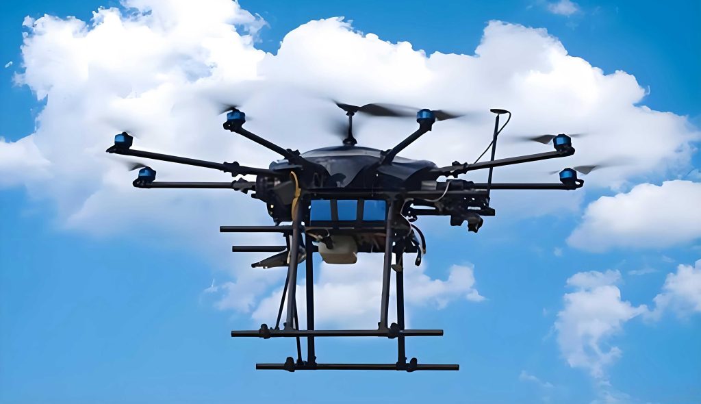
The development of intelligent connected vehicles has become a cornerstone of modern intelligent transportation systems. However, the single-vehicle perception system is often limited by line-of-sight constraints, building occlusions, and adverse weather conditions, leading to insufficient blind spot coverage and delayed responses to sudden events. To overcome these limitations, we propose to employ UAV drones as aerial mobile sensing nodes to build an air-ground integrated collaborative perception system. UAV drones offer high mobility, a global field of view, and freedom from ground traffic constraints, which can effectively compensate for the spatial limitations of ICV perception. The implementation of regulations such as the “Interim Regulations on the Flight Management of Unmanned Aerial Vehicles” and the large-scale promotion of “vehicle-road-cloud integration” technology provide policy and technical support for the collaboration between UAV drones and ICVs.
Existing studies have explored collaborative perception frameworks, path planning algorithms, and multi-agent reinforcement learning for vehicle-UAV systems. However, most prior work treats collaborative perception and path decision-making as separate problems, leading to insufficient coupling between perception information and decision optimization. Moreover, in multi-vehicle multi-UAV scenarios, existing methods cannot simultaneously adapt to the real-time scheduling of perception tasks and the integrated path planning of vehicles and UAV drones in dynamic traffic environments. To fill these gaps, we propose a two-layer collaborative optimization framework. The upper layer uses a multi-agent proximal policy optimization (MAPPO) algorithm to dynamically assign perception tasks among multiple UAV drones and ICVs. The lower layer employs an improved jump point search (JPS) algorithm to plan optimal paths for each vehicle-UAV pair under multiple constraints. This approach achieves closed-loop optimization from perception to decision-making.
2. System Modeling for Vehicle-UAV Cooperative System
2.1 Core Operation Modes
The vehicle-UAV cooperative system involves two typical operation modes: companion mode and pre-positioning mode. In companion mode, the UAV drone follows the ICV synchronously within a predefined airspace above the vehicle, collecting environmental information around the vehicle to compensate for blind spots in the front, rear, and sides. In pre-positioning mode, the UAV drone flies ahead to the front section of the planned route to acquire beyond-line-of-sight traffic information such as intersection blind spots, accidents, and congestion, providing prior information for global route replanning and local decision adjustments. According to the airspace management regulations, the low-altitude airspace from ground to 120 m is divided into three vertical flight layers, with 30–80 m designated as the dedicated collaborative perception airspace for UAV drones. Horizontally, the urban road network is divided into grid cells to form an airspace management system of “vertical layering + road network partitioning,” ensuring spatial decoupling and safety isolation between UAV flight and ground traffic operations.
2.2 Grid-Based Air-Ground Discrete Modeling
We use the grid method to discretize the urban ground traffic environment and the low-altitude perception airspace into a three-dimensional grid map. Let the planar range of the urban study area be \(X \in [0,X_{\max}]\), \(Y \in [0,Y_{\max}]\), and the vertical height range be \(Z \in [0,Z_{\max}]\). The area is divided into \(N_x \times N_y \times N_z\) cubic grids with side length \(L\), where the number of grids in each direction is given by:
$$
N_x = \frac{X_{\max}}{L}, \quad N_y = \frac{Y_{\max}}{L}, \quad N_z = \frac{Z_{\max}}{L}
$$
The grid state value \(S(x,y,z)\) characterizes both passability and perception attributes: \(S=0\) indicates a traversable/perceivable area; \(S=1\) indicates ground obstacles/buildings; \(S=2\) indicates no-fly zones/traffic control areas; \(S=3\) indicates perception blind spots. The ICV can only travel on grids with \(S=0\) at the ground level \(Z=0\), while the UAV drone can only fly in grids with \(S=0\), thereby representing ground traffic constraints, airspace constraints, obstacles, and perception blind spots in a digitized form.
2.3 Global Risk Map Construction
We classify the cooperative operation risks into three categories: ground traffic risk, aerial flight risk, and perception blind spot risk. By weighted superposition of multiple layers, we construct a global risk map that provides refined safety constraints for path decision-making. The five core risk layers are defined as follows:
1) Traffic Density Distribution Layer: Represents the impact of ground traffic congestion on vehicle passage and UAV perception. The traffic density risk value at point \((x,y)\) is:
$$
R_{\text{tra}}(x,y) = \sum_{i=1}^{n} \frac{p_i}{1+d_i}
$$
where \(p_i\) is the traffic density of the \(i\)-th grid and \(d_i\) is the distance from the target point to the center of that grid.
2) Traffic Risk Point Layer: For high-risk areas such as intersections, accident black spots, schools, and hospitals, weights are assigned according to risk levels combined with a time factor:
$$
R_{\text{risk}}(x,y) = \sum_{k} \frac{\omega_k \mu_t}{1+d_k}
$$
where \(\omega_k\) is the area type weight (1 for high risk, 0.5 for medium risk, 0.2 for low risk), \(\mu_t\) is the time factor (1.0 at peak hours, 0.6 at off-peak, 0.3 at night), and \(d_k\) is the distance from the target point to the boundary of the risk area.
3) Obstacle and No-Fly Zone Layer: Uses a decay function to define risk penalties for obstacles and no-fly zones, with gradient risks in the buffer around obstacles and outside the no-fly zone boundary:
$$
R_{\text{obs}}(x,y) = \lambda \cdot e^{-d_{\text{obs}}} + \lambda_f \cdot e^{-d_f}
$$
where \(d_{\text{obs}}\) is the distance to the nearest obstacle, \(d_f\) is the distance to the nearest no-fly zone boundary, and \(\lambda, \lambda_f\) are decay coefficients in [0.1, 1.0].
4) Perception Blind Spot Risk Layer: Quantifies the blind spot risk based on the single-vehicle perception range and building occlusion:
$$
R_{\text{blind}}(x,y) = \omega_b \cdot \frac{S_{\text{blind}}}{S_{\text{total}}}
$$
where \(S_{\text{blind}}\) is the blind spot area around the target point, \(S_{\text{total}}\) is the total perception area, and \(\omega_b\) is the blind spot risk weight.
5) Airspace Operation Risk Layer: Models collision risk and signal interference risk for low-altitude UAV drones:
$$
R_{\text{air}}(x,y,z) = \omega_{\text{air1}} \cdot e^{-d_{\text{air}}} + \omega_{\text{air2}} \cdot |z – Z_0|
$$
where \(d_{\text{air}}\) is the distance to other flying units, \(Z_0\) is the optimal perception flight height, and \(\omega_{\text{air1}}, \omega_{\text{air2}}\) are risk weights.
The normalized risk values of the above five layers are weighted and superimposed to obtain the global comprehensive risk value:
$$
R_{\text{total}}(x,y,z) = \omega_1 R_{\text{tra}} + \omega_2 R_{\text{risk}} + \omega_3 R_{\text{obs}} + \omega_4 R_{\text{blind}} + \omega_5 R_{\text{air}}
$$
where \(\omega_1\) to \(\omega_5\) sum to 1, generating the global risk map that serves as the safety constraint for collaborative perception and path decision-making.
2.4 UAV Node Layout Optimization Based on P-Median Model
UAV drone takeoff/landing and parking nodes are core infrastructure of the cooperative system. We use the P-median model to optimize node layout, with the goal of selecting P construction sites from candidate nodes to maximize the perception coverage of the entire road network while minimizing the total weighted distance cost from vehicles to the nearest service node.
Objective function:
$$
\min \quad Z = \sum_{j \in J} f_j y_j + \sum_{i \in I} \sum_{j \in J} c_{ij} q_i d_{ij} x_{ij}
$$
$$
\max \quad S_{\text{cover}} = \frac{\sum_{i \in I} S_{\text{cover}}(i)}{S_{\text{total}}}
$$
where \(I\) is the set of road network demand points, \(J\) is the set of candidate nodes, \(f_j\) is the fixed construction cost of candidate node \(j\), \(c_{ij}\) is the transportation cost per km from node \(j\) to demand point \(i\), \(d_{ij}\) is the flight distance, \(q_i\) is the traffic volume at demand point \(i\), \(S_{\text{cover}}(i)\) is the perception coverage area at demand point \(i\), and \(S_{\text{total}}\) is the total study area.
Decision variables: \(y_j \in \{0,1\}\) (1 if candidate node \(j\) is selected), \(x_{ij} \in \{0,1\}\) (1 if demand point \(i\) is served by node \(j\)).
Constraints:
$$
\begin{aligned}
&\sum_{j \in J} x_{ij} = 1, \quad \forall i \in I \\
&x_{ij} \leq y_j, \quad \forall i \in I, j \in J \\
&\sum_{j \in J} y_j = P \\
&\sum_{i \in I} q_i x_{ij} \leq Q_{\max}, \quad \forall j \in J \\
&d_{ij} \leq D_{\max}, \quad \forall i \in I, j \in J \\
&d_{jj’} \geq D_{\min}, \quad \forall j, j’ \in J, j \neq j’
\end{aligned}
$$
Constraint (1) ensures each demand point is served by exactly one node; (2) ensures a demand point is served only by a selected node; (3) limits the number of selected nodes to \(P\); (4) limits the maximum carrying capacity of each node; (5) limits the maximum single flight distance of UAV drones; (6) ensures a minimum safe distance between nodes.
2.5 Problem Statement
The core problem addressed in this paper is to design a two-layer optimization method for a multi-UAV multi-ICV cooperative system in complex urban traffic environments, aiming at closed-loop “perception-decision” optimization. The upper layer uses multi-agent reinforcement learning to dynamically assign collaborative perception tasks optimally, completing the matching and scheduling of UAV drones and ICVs. The lower layer, based on an improved path search algorithm, plans an integrated optimal path for each vehicle-UAV pair that satisfies multiple constraints, ultimately achieving the goals of maximizing perception coverage and minimizing comprehensive traffic cost.
3. Multi-Objective Path Decision-Making Optimization Model
3.1 Objective Function Construction
Considering perception coverage, traffic efficiency, collaborative cost, and energy consumption, we construct the total cost objective function:
$$
\min \quad J = \omega_1 C_{\text{cover}} + \omega_2 F_{\text{vehicle}} + \omega_3 F_{\text{UAV}} + \omega_4 F_{\text{cost}}
$$
where \(\omega_1, \omega_2, \omega_3, \omega_4\) are weight coefficients satisfying \(\omega_1+\omega_2+\omega_3+\omega_4=1\). \(C_{\text{cover}}\) is the global perception coverage.
1) Perception Coverage Objective: Measures the effectiveness of vehicle-UAV cooperation:
$$
C_{\text{cover}} = \frac{S_{\text{vehicle}} \cup S_{\text{UAV}}}{S_{\text{target}}} \times 100\%
$$
where \(S_{\text{vehicle}}\) is the single-vehicle perception coverage area, \(S_{\text{UAV}}\) is the UAV drone perception coverage area, and \(S_{\text{target}}\) is the total area of the target road segment.
2) Vehicle Traffic Cost: Considers path length, travel time, and traffic risk:
$$
F_{\text{vehicle}} = \sum_{k=1}^{n-1} \left( \alpha_1 l_k + \alpha_2 t_k + \alpha_3 R_{\text{road}}(k) \right)
$$
where \(l_k\) is the path length between adjacent nodes, \(t_k\) is the travel time on that segment, \(R_{\text{road}}(k)\) is the ground comprehensive risk value at node \(k\), and \(\alpha_1, \alpha_2, \alpha_3\) are weights.
3) UAV Flight Cost: Considers flight distance, energy consumption, and air risk:
$$
F_{\text{UAV}} = \sum_{k=1}^{m-1} \left( \beta_1 d_k + \beta_2 e_k + \beta_3 R_{\text{air}}(k) \right)
$$
where \(d_k\) is the flight distance between adjacent nodes, \(e_k\) is the energy consumption on that segment, \(R_{\text{air}}(k)\) is the airspace risk value at node \(k\), and \(\beta_1, \beta_2, \beta_3\) are weights.
4) Collaborative Cost: Represents the comprehensive cost of vehicle-UAV communication, time synchronization, and task scheduling:
$$
F_{\text{cost}} = \gamma_1 |t_{\text{vehicle}} – t_{\text{UAV}}| + \gamma_2 n_{\text{task}}
$$
where \(t_{\text{vehicle}}\) is the time for the vehicle to reach the target node, \(t_{\text{UAV}}\) is the time for the UAV drone to reach the corresponding node, \(n_{\text{task}}\) is the number of perception task scheduling times, and \(\gamma_1, \gamma_2\) are weights.
The weights are determined by the analytic hierarchy process (AHP). After passing the consistency test (CR=0.072<0.1), the baseline weight combination is \(\omega_1=0.4, \omega_2=0.3, \omega_3=0.2, \omega_4=0.1\). This setting follows the design principle of “safety first, efficiency balanced” for autonomous driving, referring to similar weight allocation logic in ICV path planning studies.
3.2 Multi-Constraint Setting
1) ICV Constraints:
- Vehicle dynamics: maximum speed \(v_{\max}\), acceleration range \([a_{\min}, a_{\max}]\), minimum turning radius \(R_{\min}\).
- Traffic rules: no reverse driving, no crossing solid lines, obey traffic signals.
- Collision avoidance: all path nodes must have grid state \(S=0\), maintain safe distance from dynamic obstacles.
2) UAV Drone Constraints:
- Performance: maximum range \(D_{\max}\), maximum speed \(v_{\max}\), maximum turning angle \(\theta_{\max}\), flight height limits, battery energy \(E_0\) with remaining reserve \(E_{\text{res}}\).
- Airspace: only fly in dedicated collaborative perception airspace, avoid no-fly zones, maintain safe separation from other flying units.
- Perception: flight path must meet sensor coverage requirements for target road segments, horizontal distance to the cooperative vehicle must not exceed maximum communication range.
3) Vehicle-UAV Cooperative Constraints:
- Communication: distance between vehicle and UAV drone must not exceed \(D_{\text{commax}}\).
- Time synchronization: time deviation at path nodes must not exceed maximum allowed threshold \(T_{\max}\).
- Perception synergy: UAV drone perception range must cover blind spots and high-risk sections along the vehicle’s path.
4. Two-Layer Collaborative Perception and Path Decision-Making Algorithm
We design a nested two-layer collaborative optimization algorithm: the upper layer uses MAPPO algorithm to dynamically assign multi-vehicle multi-UAV collaborative perception tasks, and the lower layer uses an improved JPS algorithm to achieve precise vehicle-UAV integrated path decision-making.
4.1 Improved JPS Algorithm
To address the rigidity of traditional JPS in dynamic traffic environments and its poor adaptability to vehicle-UAV cooperative constraints, we improve it in four aspects: bidirectional search, dynamic target following, heuristic function optimization, and path smoothing.
Bidirectional Search: Two open lists, \(open_{\text{start}}\) and \(open_{\text{end}}\), are maintained from the vehicle start and end points respectively. In each iteration, the node with the smallest cost is taken from both lists for jump point expansion. When the bidirectional searches meet, the paths are concatenated. The cost functions are:
$$
f_{\text{start}}(n) = g_{\text{start}}(n) + h_{\text{start}}(n)
$$
$$
f_{\text{end}}(m) = g_{\text{end}}(m) + h_{\text{end}}(m)
$$
where \(g_{\text{start}}(n)\) is the actual cost from start to node \(n\), \(h_{\text{start}}(n)\) is the heuristic cost from \(n\) to the end, and similarly for the reverse direction.
Dynamic Target Following: For the vehicle path search, the temporary target is set to the optimal forward node perceived in real time by the UAV drone. For the UAV drone path search, the temporary target is the vehicle’s real-time position and predicted future position. After each search iteration, the temporary target is dynamically updated based on the real-time states of the vehicle and UAV drone, allowing the algorithm to flexibly adjust the search direction in dynamic traffic environments.
Heuristic Function Optimization: Based on the Euclidean distance heuristic, we add global risk value and perception coverage constraints:
$$
h(n) = \mu_1 d(n, end) + \mu_2 R_{\text{total}}(n) + \mu_3 \frac{1}{C_{\text{cover}}(n)}
$$
where \(d(n, end)\) is the Euclidean distance from node \(n\) to the end, \(C_{\text{cover}}(n)\) is the perception coverage at node \(n\), and \(\mu_1, \mu_2, \mu_3\) are weights.
Path Smoothing: After obtaining the initial path, two optimization steps are applied: (1) vehicle path smoothing via B-spline curve fitting to eliminate sharp turns, ensuring compliance with vehicle dynamics; (2) UAV companion path optimization, breaking the limitation of straight/diagonal search, to adjust the UAV drone’s flight trajectory based on the vehicle path, ensuring the UAV stays at the optimal sensing position while reducing turns and energy consumption.
4.2 Upper-Layer Collaborative Task Allocation Based on MAPPO
For multi-UAV multi-ICV scenarios, we design a MAPPO-based algorithm for dynamic collaborative perception task allocation.
State Space: Integrates vehicle state, UAV state, traffic environment, and task information:
$$
s = [V_{\text{state}}, U_{\text{state}}, E_{\text{env}}, T_{\text{task}}]
$$
where \(V_{\text{state}}\) includes vehicle position, speed, remaining battery, perception range, and planned path; \(U_{\text{state}}\) includes UAV position, flight speed, remaining battery, perception range, and current task status; \(E_{\text{env}}\) includes global traffic density, obstacle distribution, traffic risk points, and airspace constraints; \(T_{\text{task}}\) includes perception tasks to be assigned (position, priority, time window, coverage requirements).
Action Space: Discrete action space of matching combinations between UAV drones, vehicles, and tasks:
$$
A = \{(U_j, V_i, T_k) | j \in [1,N_u], i \in [1,N_v], k \in [1,N_t]\}
$$
Each triple \((U_j, V_i, T_k)\) represents assigning the \(k\)-th perception task to the \(j\)-th UAV drone to serve the \(i\)-th ICV.
Reward Function: Designed to optimize overall cooperative performance, combining immediate and terminal rewards:
$$
R = R_{\text{cover}} + R_{\text{eff}} – R_{\text{cost}} – R_{\text{punish}}
$$
where \(R_{\text{cover}}\) is perception coverage reward, \(R_{\text{eff}}\) is traffic efficiency reward, \(R_{\text{cost}}\) is collaborative cost penalty, and \(R_{\text{punish}}\) is violation penalty.
5. Simulation Experiments and Results Analysis
5.1 Simulation Setup
We built simulation experiments based on MATLAB/Simulink platform combined with Prescan traffic simulation software. The ICV parameters reference Tesla Model 3 autonomous driving version, and the UAV drone parameters reference DJI M300 RTK industry version. Key parameters are listed in Table 1.
| Category | Parameter | Value |
|---|---|---|
| Vehicle Performance | Maximum speed (km/h) | 60 |
| Maximum acceleration (m/s²) | 3 | |
| Maximum deceleration (m/s²) | 8 | |
| Minimum turning radius (m) | 5 | |
| Single-vehicle perception range (m) | 200 | |
| UAV Drone Performance | Maximum cruise speed (m/s) | 15 |
| Maximum range (km) | 30 | |
| Maximum flight time (min) | 55 | |
| Perception coverage radius (m) | 500 | |
| Cooperative Parameters | Maximum communication distance (m) | 1000 |
| Optimal perception height (m) | 50 | |
| Maximum allowed time deviation (s) | 2 | |
| Safe obstacle avoidance distance (m) | 30 |
Two types of simulation scenarios are set: (1) Medium-density urban scenario: 3 km × 3 km area, 4 main roads, 8 secondary roads, 12 intersections, moderate traffic density, 30% obstacle coverage, 2 ICVs and 2 UAV drones; (2) High-density urban scenario: 5 km × 5 km area, 6 main roads, 15 secondary roads, 24 intersections, including schools, hospitals, commercial areas, high traffic density, 50% obstacle coverage, 5 ICVs and 4 UAV drones.
5.2 Algorithm Performance Comparison
To validate the performance of the improved JPS algorithm, we conducted single-vehicle single-UAV cooperative path decision-making experiments in both scenarios, comparing with traditional A*, Whale Optimization Algorithm (WOA), Grey Wolf Optimizer (GWO), and Particle Swarm Optimization (PSO). Each algorithm was run 20 times per scenario, and the average results are shown in Table 2 and Table 3. The comprehensive traffic cost is calculated by min-max normalization of each sub-item and weighted summation with the baseline weights (Eq. (10)).
| Algorithm | Vehicle Path Length (m) | Planning Time (s) | Perception Coverage | Comprehensive Cost |
|---|---|---|---|---|
| A* | 2864.32 | 2.12 | 72.35% | 142.68 |
| WOA | 2812.57 | 1.26 | 76.48% | 137.59 |
| GWO | 2798.43 | 1.15 | 77.62% | 135.84 |
| PSO | 2805.69 | 1.32 | 75.93% | 138.26 |
| Improved JPS | 2756.81 | 1.08 | 90.27% | 131.25 |
| Algorithm | Vehicle Path Length (m) | Planning Time (s) | Perception Coverage | Comprehensive Cost |
|---|---|---|---|---|
| A* | 5638.74 | 9.36 | 65.28% | 297.43 |
| WOA | 5726.31 | 6.92 | 68.74% | 291.56 |
| GWO | 5612.85 | 8.05 | 71.36% | 283.47 |
| PSO | 5703.49 | 8.24 | 69.52% | 289.62 |
| Improved JPS | 5482.36 | 6.71 | 84.92% | 279.14 |
In the medium-density scenario, the improved JPS algorithm reduces path length by 3.75%, planning time by 49.06%, increases perception coverage by 24.77%, and reduces comprehensive cost by 8.01% compared to traditional A*. In the high-density scenario, the improved JPS reduces path length by 2.77%, planning time by 28.32%, increases perception coverage by 19.64%, and reduces comprehensive cost by 6.15% compared to A*. Compared to swarm intelligence algorithms, the improved JPS shows significant advantages in perceptual coverage, path length, and comprehensive cost, demonstrating its robustness in complex urban traffic environments.
5.3 Sensitivity Analysis of Weight Coefficients
To analyze the impact of weight coefficients on planning results, we conducted 20 repeated experiments with four different weight combinations in the high-density scenario. The results are shown in Table 4.
| Group | ω₁ | ω₂ | ω₃ | ω₄ | Avg Path Length (m) | Avg Perception Coverage | Avg Comprehensive Cost |
|---|---|---|---|---|---|---|---|
| A | 0.5 | 0.3 | 0.1 | 0.1 | 5526.47 | 86.35% | 282.64 |
| B | 0.4 | 0.3 | 0.2 | 0.1 | 5482.36 | 84.92% | 279.14 |
| C | 0.3 | 0.4 | 0.2 | 0.1 | 5457.82 | 78.64% | 283.75 |
| D | 0.2 | 0.5 | 0.2 | 0.1 | 5432.19 | 72.38% | 288.46 |
As the weight of perception coverage (ω₁) decreases and the weight of vehicle traffic cost (ω₂) increases, the vehicle path length gradually reduces, but perception coverage decreases significantly, and the comprehensive cost first decreases and then increases. The best overall performance is achieved when ω₁=0.4, ω₂=0.3, ω₃=0.2, ω₄=0.1, balancing perception coverage, traffic efficiency, UAV flight cost, and collaborative cost. This provides a reference for weight settings in urban vehicle-UAV cooperative scenarios.
6. Conclusion
Through multi-scenario simulation experiments, we draw the following conclusions. The vehicle-UAV cooperative global risk map integrating traffic density, traffic risk points, airspace constraints, perception blind spots, and obstacle information can effectively quantify the operational risk of complex urban scenes and provide refined safety constraints for collaborative perception and path decision-making. The UAV drone node layout method based on the P-median model improves global perception coverage by 17.32% and reduces the average service distance by 10.47% compared to a uniform layout scheme, achieving optimal configuration of cooperative infrastructure. The improved JPS algorithm, through bidirectional search, dynamic target following, heuristic function optimization, and path smoothing, significantly improves the efficiency and performance of vehicle-UAV integrated path decision-making. In high-density urban scenarios, compared to the traditional A* algorithm, the path decision-making time is reduced by 28.32%, global perception coverage is improved by 19.64%, and comprehensive traffic cost is reduced by 6.15%, effectively adapting to the vehicle-UAV cooperative path decision-making needs in dynamic urban traffic environments.
Our proposed vehicle-UAV cooperative method has only been validated through simulation in conventional medium- and high-density traffic scenarios. Its robustness under extreme weather, dynamic sudden traffic events, and other extreme conditions has not been fully verified. Furthermore, the centralized training framework of the algorithm imposes high computational requirements, and the weight parameters lack scene-adaptive adjustment capabilities. Future work will focus on expanding the validation to more challenging scenarios, developing decentralized training approaches, and designing adaptive weight adjustment mechanisms to enhance the practical applicability of the system.