The evolution of unmanned aerial systems continuously pushes the boundaries of mission capability, demanding platforms that are both highly efficient and exceptionally agile. Among these, the Vertical Take-Off and Landing (VTOL) drone represents a pivotal design, merging the runway independence of rotorcraft with the aerodynamic efficiency and high-speed endurance of fixed-wing aircraft. In particular, the tail-sitting VTOL configuration offers a mechanically elegant solution, rotating its entire airframe for transition between hover and forward flight. To further enhance the agility and high-angle-of-attack performance of such a platform, the integration of a canard foreplane creates a uniquely capable VTOL drone. This paper delves into the control challenge inherent to this advanced configuration: high-speed, precise trajectory tracking in complex environments. I present a comprehensive control solution based on Model Predictive Contouring Control (MPCC), designed to navigate the inherent trade-off between tracking accuracy and aggressive forward velocity for a canard-equipped tail-sitting VTOL drone.
Traditional linear control methods, such as PID or LQR, while robust for many applications, often struggle with the highly nonlinear dynamics encountered during aggressive maneuvering or transition phases of a VTOL drone. Their reactive nature, based solely on current state error, can lead to performance degradation when tracking complex trajectories at high speeds due to system latency and model mismatch. Model Predictive Control (MPC) offers a promising framework by optimizing future control inputs over a receding horizon, explicitly handling constraints. However, a standard MPC formulation for trajectory tracking typically minimizes the Euclidean distance to a time-parameterized reference, which can unnecessarily penalize progress along the path. For a high-performance VTOL drone, the primary objectives are twofold: minimize spatial deviation from a desired path (contour error) and maximize the speed at which the path is traversed. The Model Predictive Contouring Control (MPCC) framework elegantly encodes this dual objective. My work adapts and implements this MPCC strategy for the specific, nonlinear dynamics of a canard VTOL drone, transforming the optimization problem into a tractable convex Quadratic Program (QP) for real-time feasibility.
Dynamical Model of the Canard Tail-Sitting VTOL Drone
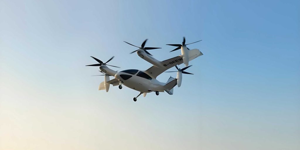
The foundation of any model-based predictive controller is a sufficiently accurate dynamical model. The vehicle under consideration is a tail-sitter with a canard, main wings, and two propellers. Its motion is described by a 6-DOF rigid-body model. The state vector is defined as:
$$
\mathbf{x} = [x_r, y_r, z_r, \phi, \theta, \psi, v_x, v_y, v_z, \omega_x, \omega_y, \omega_z, \tau]^T
$$
where $[x_r, y_r, z_r]^T$ is the position in the inertial frame, $[\phi, \theta, \psi]^T$ are the Euler angles (roll, pitch, yaw), $[v_x, v_y, v_z]^T$ is the body-frame velocity vector, $[\omega_x, \omega_y, \omega_z]^T$ is the body-frame angular rate vector, and $\tau$ is the path length variable, a virtual state introduced for the MPCC formulation.
The control input vector for this VTOL drone is:
$$
\mathbf{u} = [\delta_{al}, \delta_{ar}, \delta_{c}, u_{pl}, u_{pr}, v_{\tau}]^T
$$
Here, $\delta_{al}$ and $\delta_{ar}$ are the left and right aileron deflections (on the main wings), $\delta_{c}$ is the canard deflection, $u_{pl}$ and $u_{pr}$ are the thrust commands for the left and right propellers, and $v_{\tau}$ is the virtual speed along the path, serving as an additional control input to progress the reference.
The nonlinear dynamics are derived from Newton-Euler equations:
Translational Kinematics:
$$
\begin{bmatrix} \dot{x}_r \\ \dot{y}_r \\ \dot{z}_r \end{bmatrix} = \mathbf{R}_{BI} \begin{bmatrix} v_x \\ v_y \\ v_z \end{bmatrix}
$$
Translational Dynamics:
$$
\begin{bmatrix} \dot{v}_x \\ \dot{v}_y \\ \dot{v}_z \end{bmatrix} = \begin{bmatrix} \omega_y v_z – \omega_z v_y \\ \omega_z v_x – \omega_x v_z \\ \omega_x v_y – \omega_y v_x \end{bmatrix} + \frac{1}{m} \mathbf{f}
$$
Rotational Kinematics:
$$
\begin{bmatrix} \dot{\phi} \\ \dot{\theta} \\ \dot{\psi} \end{bmatrix} = \begin{bmatrix}
1 & \sin\phi \tan\theta & \cos\phi \tan\theta \\
0 & \cos\phi & -\sin\phi \\
0 & \sin\phi / \cos\theta & \cos\phi / \cos\theta
\end{bmatrix} \begin{bmatrix} \omega_x \\ \omega_y \\ \omega_z \end{bmatrix}
$$
Rotational Dynamics:
$$
\begin{bmatrix} \dot{\omega}_x \\ \dot{\omega}_y \\ \dot{\omega}_z \end{bmatrix} = \mathbf{J}^{-1} \left( \mathbf{m} – \boldsymbol{\omega} \times \mathbf{J} \boldsymbol{\omega} \right)
$$
where $\mathbf{R}_{BI}$ is the rotation matrix from body to inertial frame, $m$ is the mass, $\mathbf{J}$ is the inertia tensor, $\mathbf{f}$ is the total force vector, and $\mathbf{m}$ is the total moment vector, both expressed in the body frame. The forces and moments are summations of contributions from gravity, aerodynamics on the canard and main wings, and propeller thrust. The aerodynamic forces are modeled as functions of airspeed, angle of attack, and control surface deflections. A key parameter set for the modeled VTOL drone is summarized below.
| Parameter | Symbol | Value | Unit |
|---|---|---|---|
| Total Mass | $m$ | 1.43 | kg |
| Wingspan | $b$ | 1.20 | m |
| Cruise Speed | $V_c$ | 12.0 | m/s |
| Max Lift-to-Drag Ratio | $(L/D)_{max}$ | 10.5 | – |
| Hover Thrust-to-Weight Ratio | $T/W$ | 2.01 | – |
Trajectory Parameterization and MPCC Problem Formulation
The core innovation of the MPCC approach lies in its treatment of the reference trajectory. Instead of a time-parametrized path $\mathbf{p}_d(t)$, we consider a geometric path parameterized by its arc length $\tau$: $\mathbf{p}_d(\tau) = [x_d(\tau), y_d(\tau), z_d(\tau)]^T$. A given set of waypoints is interpolated using cubic splines and then re-parameterized by $\tau$. The virtual state $\tau$ evolves according to $\dot{\tau} = v_{\tau}$, where $v_{\tau}$ is a controlled variable. This decouples the timing of the reference from the spatial path, allowing the controller to decide how fast to move along it.
The core tracking errors in MPCC are defined geometrically, as illustrated in the figure below. Let $\mathbf{p}_k$ be the vehicle’s position at step $k$ and $\mathbf{p}_d(\hat{\tau}_k)$ be the point on the path corresponding to the current arc length estimate $\hat{\tau}_k$. The lag error $e_l$ is the component of the vector $\mathbf{e} = \mathbf{p}_k – \mathbf{p}_d(\hat{\tau}_k)$ that is tangential to the path. The contour error $e_c$ is the component normal to the path. Minimizing $e_c$ keeps the VTOL drone close to the desired geometry, while minimizing $e_l$ ensures the estimated arc length $\hat{\tau}_k$ stays synchronized with the closest point on the path. Maximizing $v_{\tau}$ encourages fast progression.
The complete nonlinear MPCC optimization problem over a prediction horizon $N$ is formulated as follows:
$$
\begin{aligned}
\min_{\mathbf{u}_{0:N-1}} & \sum_{k=0}^{N-1} \left( \underbrace{q_l \| e_l(\hat{\tau}_k) \|^2}_{\text{Lag Error}} + \underbrace{q_c \| e_c(\hat{\tau}_k) \|^2}_{\text{Contour Error}} + \underbrace{\Delta\mathbf{u}_k^T \mathbf{R} \Delta\mathbf{u}_k}_{\text{Input Smoothing}} – \underbrace{\beta v_{\tau, k}}_{\text{Progress}} \right) \\
\text{subject to: } & \mathbf{x}_{0} = \mathbf{x}_{\text{init}} \\
& \mathbf{x}_{k+1} = f(\mathbf{x}_k, \mathbf{u}_k), \quad k = 0,…,N-1 \\
& \mathbf{x}_{min} \leq \mathbf{x}_k \leq \mathbf{x}_{max} \\
& \mathbf{u}_{min} \leq \mathbf{u}_k \leq \mathbf{u}_{max} \\
& 0 \leq v_{\tau, k} \leq \bar{v}_{\tau}
\end{aligned}
$$
Here, $q_l$, $q_c$, and $\beta$ are tunable weight parameters that balance the competing objectives of lag minimization, contour accuracy, and speed, respectively. $\mathbf{R}$ penalizes aggressive control changes. This formulation directly addresses the high-speed tracking challenge for a VTOL drone by making the speed-vs-accuracy trade-off explicit and tunable.
Linearization and Convex Quadratic Programming Solution
Solving the nonlinear MPCC problem in real-time is computationally prohibitive for a fast-paced VTOL drone. To achieve real-time performance, I employ a successive linearization approach, transforming the problem into a convex Quadratic Program (QP) at each control step.
First, the nonlinear dynamics $f(\mathbf{x}_k, \mathbf{u}_k)$ are linearized around the current state and input trajectory $(\bar{\mathbf{x}}_k, \bar{\mathbf{u}}_k)$ from the previous solution (or an initial guess):
$$
\mathbf{x}_{k+1} \approx f(\bar{\mathbf{x}}_k, \bar{\mathbf{u}}_k) + \mathbf{A}_k (\mathbf{x}_k – \bar{\mathbf{x}}_k) + \mathbf{B}_k (\mathbf{u}_k – \bar{\mathbf{u}}_k)
$$
where $\mathbf{A}_k = \frac{\partial f}{\partial \mathbf{x}} \big|_{\bar{\mathbf{x}}_k, \bar{\mathbf{u}}_k}$ and $\mathbf{B}_k = \frac{\partial f}{\partial \mathbf{u}} \big|_{\bar{\mathbf{x}}_k, \bar{\mathbf{u}}_k}$ are the Jacobian matrices. This yields a linear time-varying (LTV) model constraint: $\mathbf{x}_{k+1} = \mathbf{A}_k \mathbf{x}_k + \mathbf{B}_k \mathbf{u}_k + \mathbf{g}_k$.
Second, the contour and lag error terms in the cost function are also linearized. The errors $e_c$ and $e_l$ are functions of the state $\mathbf{x}_k$ (specifically the position and the arc length $\tau_k$). Their quadratic forms are approximated by linearizing around the same operating point:
$$
\|e(\bar{\mathbf{x}}_k)\|^2 \approx \|e(\bar{\mathbf{x}}_k)\|^2 + 2 e(\bar{\mathbf{x}}_k)^T \frac{\partial e}{\partial \mathbf{x}} \big|_{\bar{\mathbf{x}}_k} (\mathbf{x}_k – \bar{\mathbf{x}}_k) + (\mathbf{x}_k – \bar{\mathbf{x}}_k)^T \left( \frac{\partial e}{\partial \mathbf{x}}^T \frac{\partial e}{\partial \mathbf{x}} \right) \big|_{\bar{\mathbf{x}}_k} (\mathbf{x}_k – \bar{\mathbf{x}}_k)
$$
After these linearizations, the original MPCC problem is approximated by the following QP at each time step:
$$
\begin{aligned}
\min_{\mathbf{X}, \mathbf{U}} & \quad \frac{1}{2} \begin{bmatrix} \mathbf{X} \\ \mathbf{U} \end{bmatrix}^T \mathbf{H} \begin{bmatrix} \mathbf{X} \\ \mathbf{U} \end{bmatrix} + \mathbf{c}^T \begin{bmatrix} \mathbf{X} \\ \mathbf{U} \end{bmatrix} \\
\text{s.t.} & \quad \mathbf{x}_0 = \mathbf{x}(t_0) \\
& \quad \mathbf{x}_{k+1} = \mathbf{A}_k \mathbf{x}_k + \mathbf{B}_k \mathbf{u}_k + \mathbf{g}_k, \quad \forall k \\
& \quad \mathbf{x}_{min} \leq \mathbf{x}_k \leq \mathbf{x}_{max} \\
& \quad \mathbf{u}_{min} \leq \mathbf{u}_k \leq \mathbf{u}_{max}
\end{aligned}
$$
Here, $\mathbf{X} = [\mathbf{x}_0^T, …, \mathbf{x}_N^T]^T$ and $\mathbf{U} = [\mathbf{u}_0^T, …, \mathbf{u}_{N-1}^T]^T$ are the stacked state and input sequences over the horizon. The matrix $\mathbf{H}$ is constructed from the quadratic terms of the linearized errors and the input smoothing term, ensuring convexity (positive semi-definiteness). The vector $\mathbf{c}$ contains the linear terms from the error linearization and the progress term $-\beta v_{\tau}$. This QP can be solved very efficiently using standard solvers. Only the first control input $\mathbf{u}_0^*$ from the optimal sequence is applied to the VTOL drone before the process repeats at the next time step with updated state feedback.
Simulation Results and Comparative Analysis
I implemented the proposed MPCC controller in a high-fidelity simulation environment to validate its performance for the canard VTOL drone. The solver uses a prediction horizon of $N=50$ steps with a time step of $\Delta t = 0.05$ s, resulting in a 2.5-second look-ahead and a 20 Hz control frequency. The key MPCC tuning parameters used in the simulations are:
| Parameter | Description | Value |
|---|---|---|
| $q_c$ | Contour error weight | 1.0 |
| $q_l$ | Lag error weight | 1000.0 |
| $\beta$ | Path progress weight | 0.5 |
| $q_{c,N}$ | Terminal contour error weight | 1000.0 |
1. Figure-Eight Tracking (Balanced Mode): The first test involves a planar figure-eight path (60m x 20m). Starting from a point on the path with initial forward speed, the MPCC controller demonstrates effective tracking. In straight segments, the VTOL drone adheres closely to the path. In turns, the controller intelligently trades a slight increase in contour error for a larger turning radius, allowing it to maintain a higher speed $v_{\tau}$. This is the desired “balanced” behavior where the drone prioritizes speed while keeping error within acceptable bounds.
2. Hover-to-Level Transition Tracking: A more complex trajectory was designed to test the full capability of the VTOL drone. It begins in a hover, climbs vertically, executes a transition to level flight, and finally follows a circular arc. The MPCC controller successfully managed this multi-phase flight, accurately tracking both the vertical ascent and the subsequent horizontal maneuver, showcasing its ability to handle the significantly different dynamics across flight regimes.
3. Small-Radius Figure-Eight (Accuracy Mode): To test performance under tight spatial constraints, a smaller figure-eight (30m x 12m) was used. With the original “balanced” weights, the tracking error became significant as the drone prioritized speed over the tight geometry. By reconfirming the controller parameters to prioritize accuracy ($q_c = 1000$, $\beta = 0.1$), the VTOL drone successfully tracked the tight path with much higher fidelity, at the cost of a 6% reduction in lap time. This highlights the critical and tunable trade-off inherent to the MPCC framework.
4. Complex Urban Canyon Scenario: A comprehensive test involved a 100m x 100m simulated urban environment with narrow passages (5m width), vertical climbs, turns, and a descending spiral. The MPCC-guided VTOL drone navigated this entire course successfully, maintaining precise tracking through narrow gates at speeds up to 15 m/s and seamlessly executing different flight phases.
5. Comparison with Standard Time-Based MPC: To quantify the advantage of the contouring approach, a standard time-based MPC was implemented for comparison on the large figure-eight track. The standard MPC aims to minimize the error to a time-parameterized reference. The results are summarized below:
| Metric | MPCC Controller | Standard MPC |
|---|---|---|
| Lap Time | 12.0 s | 18.0 s (+50%) |
| Mean Contour Error | 0.15 m | 0.22 m |
| Error Std. Dev. | 0.08 m | 0.14 m |
The MPCC controller completed the track 50% faster than the standard MPC while also achieving a lower average tracking error and significantly better error consistency (smaller standard deviation). This conclusively demonstrates that the MPCC formulation is superior for high-speed trajectory tracking tasks where progress along the path is a key objective, as is often the case for a delivery or reconnaissance VTOL drone.
Conclusion and Future Work
In this work, I have developed and validated a Model Predictive Contouring Control (MPCC) strategy for high-speed trajectory tracking of a sophisticated canard-equipped tail-sitting VTOL drone. The controller explicitly balances the dual objectives of path accuracy and forward progress through a well-designed cost function. By employing successive linearization to form a convex Quadratic Program at each time step, the algorithm achieves computational efficiency suitable for real-time implementation. Extensive simulations across various trajectory types—from simple loiters to complex urban canyons and dynamic transitions—confirm the effectiveness and versatility of the approach. The direct comparison with a standard time-based MPC underscores MPCC’s superior performance in high-speed tracking scenarios, making it a compelling solution for enhancing the autonomy of agile VTOL drone platforms.
Several avenues for future work remain open. First, the current linearization-based MPCC, while fast, is only locally optimal. Investigating more advanced nonlinear programming solvers or real-time iteration schemes could improve global performance, especially during very aggressive maneuvers. Second, the robustness of the controller to strong wind disturbances and model uncertainties needs to be formally addressed, possibly through the integration of a disturbance observer or a robust MPC formulation. Third, the transition from forward flight back to hover (the backward transition) presents unique aerodynamic challenges, including potential stall conditions, which were not covered in this model. Extending the aerodynamic model and controller to handle this regime is crucial for full mission capability. Finally, the ultimate validation step is flight testing on a physical VTOL drone prototype, which will require careful system identification to refine the aerodynamic parameters and further optimization of the control frequency and solver latency for deployment on embedded hardware.