
The proliferation and increasing sophistication of Unmanned Aerial Vehicle (UAV) technology present a formidable and evolving challenge to modern air defense paradigms. The concept of UAV swarm attacks, characterized by the coordinated deployment of numerous, often low-cost, small to medium-sized drones, has transitioned from theoretical research to a tangible tactical reality. These swarms aim to overwhelm traditional defense systems through sheer numbers, distributed intelligence, and cooperative behaviors, exploiting gaps in coverage, saturating engagement channels, and dramatically increasing the cost-exchange ratio in favor of the attacker. In this complex threat landscape, integrated missile and gun air defense systems emerge as a critical last line of defense for point and area protection. My analysis focuses on modeling and evaluating the operational effectiveness of such integrated systems in the anti-UAV swarm context. By leveraging queuing theory and combat simulations, I aim to quantify system capabilities, identify key performance parameters, and propose optimization pathways to enhance anti-UAV swarm resilience.
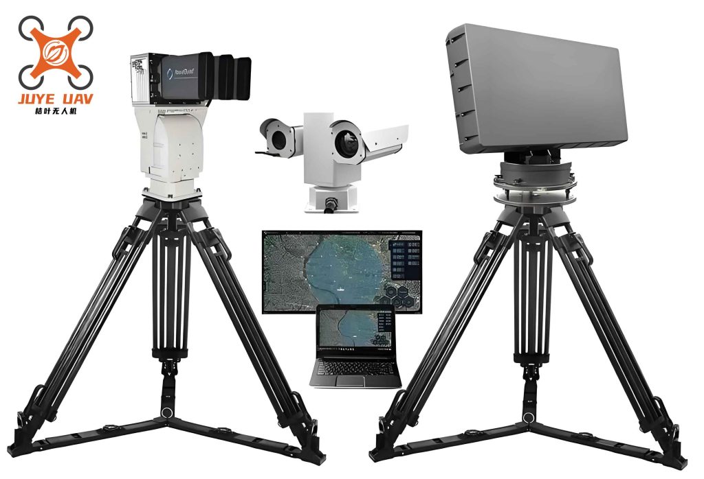
The fundamental challenge in anti-UAV swarm defense is managing a high-volume, stochastic stream of targets with limited engagement resources. A typical integrated system comprises a surveillance radar, a fire control radar, a command unit, several launchers for surface-to-air missiles (SAMs), and one or more close-in weapon systems (CIWS), typically rapid-firing guns. This combination allows for layered engagement: missiles handle targets at longer ranges and higher altitudes, while guns provide a high-rate-of-fire solution for leakers or targets that penetrate the inner zone. The system’s effectiveness against a swarm is not merely the sum of its missile and gun kill probabilities; it is a dynamic function of detection, tracking, decision-making, engagement sequencing, and reloading cycles—all under severe time constraints imposed by the swarm’s tempo.
To analytically capture this dynamic, I employ a queuing theory model, specifically an M/M/s queue with finite patience (an M/M/s + M queue). This model is apt for representing the swarm attack as a Poisson arrival process and the defense system’s engagement service times as exponential distributions. The “finite patience” represents the limited time a target remains in the weapon’s effective engagement zone before it flies through. The system has ‘s’ identical servers (engagement channels), each representing a launcher or gun turret capable of handling one target at a time.
Let’s define the key parameters for the model:
- $\lambda$: The average arrival rate of UAVs into the defense zone (targets per minute).
- $\mu$: The average service rate of an engagement channel, where $\mu = 1 / \bar{T}_{service}$. $\bar{T}_{service}$ is the mean total time to engage a target (including acquisition, aiming, firing, and assessing for the next shot).
- $s$: The number of parallel engagement channels (e.g., missile launchers + gun turrets).
- $\nu$: The abandonment rate, where $\nu = 1 / \bar{T}_{zone}$. $\bar{T}_{zone}$ is the mean time a target stays within the lethal envelope of the weapon system.
- $P_{kill,m}$: The single-shot kill probability of the missile subsystem against a UAV.
- $P_{kill,g}$: The kill probability per burst or per short engagement of the gun subsystem.
The state of the system, $P_n$, represents the probability that there are ‘n’ targets in the system (either being engaged or waiting). For $n < s$, all targets are being serviced immediately. For $n \geq s$, all ‘s’ channels are busy, and $(n-s)$ targets are in a queue. These queued targets have a finite “patience” (time in zone) before they automatically “abandon” the queue (i.e., exit the engagement zone successfully). The state transition diagram leads to the following steady-state balance equations:
For $0 \leq n < s$:
$$ \lambda P_{n-1} + (n+1)\mu P_{n+1} = (\lambda + n\mu)P_n $$
For $n \geq s$:
$$ \lambda P_{n-1} + (s\mu + (n+1-s)\nu) P_{n+1} = (\lambda + s\mu + (n-s)\nu)P_n $$
Solving these equations yields the steady-state probabilities. Let $\rho = \lambda / \mu$ and $\sigma = \nu / \mu$. The probability that the system is idle ($P_0$) is the cornerstone for calculation:
$$
P_0 = \left[ \sum_{n=0}^{s-1} \frac{\rho^n}{n!} + \frac{\rho^s}{s!} \sum_{j=0}^{\infty} \left( \frac{\rho}{s} \right)^j \prod_{k=1}^{j} \left( 1 + \frac{k\sigma}{s} \right)^{-1} \right]^{-1}
$$
Subsequent state probabilities are:
For $1 \leq n \leq s$:
$$ P_n = P_0 \frac{\rho^n}{n!} $$
For $n = s+j$ with $j \geq 1$:
$$ P_{s+j} = P_0 \frac{\rho^s}{s!} \prod_{k=1}^{j} \frac{\rho}{s + k\sigma} $$
From these probabilities, we can derive critical performance metrics for each weapon subsystem (missile and gun, treated as independent queues sharing the same arrival process but with different service rates $\mu_m$, $\mu_g$ and zone times $\nu_m$, $\nu_g$).
The key metric is the probability that a randomly arriving UAV is successfully engaged by a subsystem before it exits the zone. This is 1 minus the probability it abandons the queue. The rate at which targets abandon the queue for the missile subsystem is $\nu_m \cdot E[L_{q,m}]$, where $E[L_{q,m}]$ is the expected queue length for the missile queue. The abandonment probability $P_{ab,m}$ is this rate divided by the arrival rate $\lambda$:
$$
P_{ab,m} = \frac{\nu_m}{\lambda} \cdot E[L_{q,m}] = \frac{\nu_m}{\lambda} \sum_{j=1}^{\infty} j \cdot P_{s_m + j}
$$
Therefore, the missile subsystem’s interception probability $P_{int,m}$ is:
$$
P_{int,m} = 1 – P_{ab,m}
$$
However, interception does not guarantee kill. Accounting for the single-shot kill probability $P_{kill,m}$, the probability that a UAV is destroyed by the missile subsystem is:
$$
P_{dest,m} = P_{int,m} \cdot P_{kill,m}
$$
A similar set of equations applies to the gun subsystem, yielding $P_{dest,g}$.
Since the missile and gun engage in a layered defense, a UAV must survive both layers to penetrate. Assuming engagements are independent, the total probability of a UAV penetrating the integrated defense system $P_{pen}$ is:
$$
P_{pen} = (1 – P_{dest,m}) \cdot (1 – P_{dest,g})
$$
Consequently, the overall system kill probability $P_{kill,sys}$ is:
$$
P_{kill,sys} = 1 – P_{pen} = P_{dest,m} + P_{dest,g} – P_{dest,m} \cdot P_{dest,g}
$$
Finally, the operational capacity $N_{kill}$ of the system over a mission duration $T$ under a constant swarm arrival rate $\lambda$ is the expected number of UAVs killed:
$$
N_{kill} = \lambda \cdot T \cdot P_{kill,sys}
$$
This model forms the basis for our simulation and analysis of anti-UAV swarm capabilities.
I now present a series of simulation analyses to dissect the influence of key system parameters on anti-UAV swarm effectiveness. The baseline scenario involves a swarm of 100 small UAVs arriving over a 30-minute mission window ($T=30$ min). The integrated system has $s=6$ total engagement channels. The missiles have a mean engagement time $\bar{T}_{service,m} = 60$ seconds and a kill probability $P_{kill,m}=0.8$. The guns have a much faster mean engagement time $\bar{T}_{service,g} = 10$ seconds but a lower per-engagement kill probability $P_{kill,g}=0.4$. The zone dwell time $\bar{T}_{zone}$ is varied based on weapon range.
Analysis 1: The Impact of Missile Range (and Implicitly, Zone Dwell Time)
Missile range directly affects $\bar{T}_{zone,m}$. A longer range extends the engagement timeline, allowing more opportunities to service queued targets. We compare missiles with effective ranges of 5km, 10km, and 15km. A simplistic linear relationship is assumed: $\bar{T}_{zone,m} (min) \approx \frac{Range (km)}{Target Speed (km/min)}$. A target speed of 150 km/h (2.5 km/min) is used. Gun range is fixed at 4km.
| Simulation Parameter | Missile Range = 5 km | Missile Range = 10 km | Missile Range = 15 km |
|---|---|---|---|
| $\bar{T}_{zone,m}$ (min) | 2.0 | 4.0 | 6.0 |
| $P_{dest,m}$ (Missile Dest. Prob.) | 0.625 | 0.629 | 0.644 |
| $P_{dest,g}$ (Gun Dest. Prob.) | 0.973 | 0.973 | 0.973 |
| $P_{pen}$ (Penetration Prob.) | 0.0102 | 0.0101 | 0.0097 |
| $P_{kill,sys}$ (System Kill Prob.) | 0.9898 | 0.9899 | 0.9903 |
| $N_{kill}$ (Expected Kills) | 98.98 | 98.99 | 99.03 |
The results reveal a critical insight: while increasing missile range provides a marginal improvement in its destruction probability, the gun subsystem remains the dominant layer, achieving near-saturation interception probabilities (~0.973). This is due to its extremely high service rate ($\mu_g = 6$/min) compared to the missile’s rate ($\mu_m = 1$/min). The swarm is primarily dealt with by the guns. Therefore, for anti-UAV swarm defense, optimizing the gun subsystem is paramount. Investing in extremely long-range missiles offers diminishing returns for swarm defense compared to enhancing gun performance or increasing the number of gun channels. A balanced design with missiles covering medium ranges (e.g., 10km) to handle high-priority or faster targets, coupled with an optimized gun layer, is the most cost-effective architecture for anti-UAV operations.
Analysis 2: The Impact of Gun Kill Probability
Given the gun’s pivotal role, its kill probability per engagement $P_{kill,g}$ is a major driver of overall system effectiveness. We analyze a more stressing scenario with a 200-UAV swarm. The missile parameters remain as the 10km baseline ($P_{kill,m}=0.8$). We vary the gun’s kill probability.
| Simulation Parameter | $P_{kill,g} = 0.4$ | $P_{kill,g} = 0.6$ | $P_{kill,g} = 0.8$ |
|---|---|---|---|
| $P_{dest,m}$ | 0.597 | 0.597 | 0.597 |
| $P_{dest,g}$ | 0.733 | 0.952 | 0.997 |
| $P_{pen}$ | 0.1078 | 0.0194 | 0.0012 |
| $P_{kill,sys}$ | 0.8922 | 0.9806 | 0.9988 |
| $N_{kill}$ (Out of 200) | 178.4 | 196.1 | 199.8 |
The sensitivity is dramatic. Increasing $P_{kill,g}$ from 0.4 to 0.6 reduces expected penetrations by over 80% (from 21.6 to 3.9). This underscores that in anti-UAV swarm defense, volume of fire must be matched with high lethality per time unit. Improving $P_{kill,g}$ involves multiple factors: using optimized airburst or pre-fragmented ammunition tailored for small, agile UAVs; enhancing fire control solution accuracy (reducing aiming errors); and increasing hit probability through higher muzzle velocity or advanced guidance for smart projectiles. This parameter is a primary focus for research and development in modern anti-UAV close-in defense systems.
Analysis 3: The Impact of System Reaction and Engagement Time
The service rate $\mu$ is a function of the total engagement cycle time. Shortening this cycle directly increases the number of targets that can be serviced, reducing queue abandonment. We first examine the effect of improving the gun’s engagement cycle time $\bar{T}_{service,g}$.
| Simulation Parameter | $\bar{T}_{service,g} = 10s$ ($\mu_g=6$/min) | $\bar{T}_{service,g} = 8s$ ($\mu_g=7.5$/min) | $\bar{T}_{service,g} = 6s$ ($\mu_g=10$/min) |
|---|---|---|---|
| $P_{dest,m}$ | 0.597 | 0.597 | 0.597 |
| $P_{dest,g}$ | 0.733 | 0.785 | 0.942 |
| $P_{pen}$ | 0.1078 | 0.0865 | 0.0234 |
| $N_{kill}$ | 178.4 | 182.7 | 195.3 |
A reduction from 10 to 6 seconds, achievable through faster slewing turrets, advanced tracking algorithms, and streamlined firing sequences, yields a significant boost in kills (from 178 to 195 out of 200). This highlights the critical importance of automation and high-speed servos in anti-UAV gun systems.
While the missile subsystem plays a secondary role against dense swarms, its engagement time still matters for handling the initial wave or higher-value targets in a mixed swarm. We fix the gun at $\bar{T}_{service,g}=8s$ and vary the missile engagement time.
| Simulation Parameter | $\bar{T}_{service,m} = 60s$ ($\mu_m=1$/min) | $\bar{T}_{service,m} = 45s$ ($\mu_m=1.33$/min) | $\bar{T}_{service,m} = 30s$ ($\mu_m=2$/min) |
|---|---|---|---|
| $P_{dest,m}$ | 0.597 | 0.610 | 0.676 |
| $P_{dest,g}$ | 0.785 | 0.785 | 0.785 |
| $P_{pen}$ | 0.0865 | 0.0837 | 0.0694 |
| $N_{kill}$ | 182.7 | 183.3 | 186.1 |
Improving missile engagement time (via faster launch sequence, lock-on-after-launch capabilities, or dual-mode seekers for quick acquisition) has a measurable, though less pronounced, effect on the overall outcome because the gun layer is already highly effective. However, in scenarios with higher-fidelity or more threatening UAVs that require missile interception, reducing this cycle time is vital for maintaining a high probability of kill against the first several targets, preventing early leakage.
The mathematical modeling and simulation analyses lead to several concrete conclusions and recommendations for enhancing integrated air defense systems for the anti-UAV swarm mission:
- Prioritize the Gun Layer: Against low-cost, numerous UAV swarms, the close-in gun system is the workhorse. System architecture and resource allocation should reflect this. Investments should focus on increasing the number of gun channels (s) and boosting their individual performance ($\mu_g$, $P_{kill,g}$) before pursuing marginal improvements in missile range.
- Optimize for Lethality per Unit Time: The product of service rate and kill probability ($\mu \cdot P_{kill}$) is a key metric for both missiles and guns. For guns, this means employing advanced ammunition and precision fire control to maximize $P_{kill,g}$ without sacrificing rate of fire. For missiles, it may favor designs with slightly lower single-shot probability but much shorter engagement cycles (e.g., smaller, faster missiles with fire-and-forget or mid-course update capabilities) to increase $\mu_m$.
- Reduce Total Engagement Cycle Time: Every second saved in the detect-to-engage chain directly increases system capacity. This requires integrated, high-speed sensor suites (combining radar, electro-optical, and electronic support measures), rapid communication networks, and highly automated decision-making aids to minimize human-in-the-loop delays. Autonomic target assignment and firing are likely necessities for effective anti-UAV swarm defense.
- Employ Networked and Distributed Systems: A single integrated system, no matter how good, has a finite capacity ‘s’. The ultimate solution for large swarms is a networked cluster of such systems, creating a distributed, resilient defensive grid. Queuing models can be extended to analyze such networks, where targets can be handed off or engaged by multiple nodes, dramatically increasing the effective ‘s’ for the defended area.
- Incorporate Soft-Kill Measures: The model currently considers only kinetic kill. Integrating electronic attack (jamming, spoofing) or directed energy weapons into the service channels can be highly effective. These systems often have different service parameters (e.g., very high $\mu$ for a wide-area jammer but potentially lower $P_{kill}$ against hardened drones). A hybrid queue incorporating both hard- and soft-kill “servers” would provide a more complete optimization framework for a layered anti-UAV defense.
In conclusion, the threat of UAV swarms necessitates a rigorous, quantitative approach to air defense system design and evaluation. The queuing theory model presented here provides a powerful tool for understanding the dynamics of swarm engagements and identifying the parameters that most significantly impact an integrated system’s anti-UAV capability. The analysis unequivocally shows that success hinges on high-speed, high-lethality close-in defense, supported by efficient medium-range missiles, all orchestrated by seamless, automated command and control. By focusing engineering efforts on optimizing these key parameters—service rate and kill probability of the gun layer, and overall system reaction time—developers can create integrated air defense systems capable of providing robust protection against the evolving and pervasive challenge of UAV swarm attacks.