
In the contemporary security landscape, the proliferation of unmanned aerial vehicles (UAVs), particularly small, inexpensive, and commercially available models, presents a profound challenge to traditional air defense systems. These “low, slow, and small” (LSS) targets often evade conventional radar and radio frequency (RF) detection methods, necessitating the development of complementary and often passive sensing technologies. Among these, acoustic detection has emerged as a critical component in a layered anti-UAV defense strategy. This paper, from the perspective of a researcher in the field, provides a comprehensive overview of acoustic detection systems for countering UAV threats. While inherently limited in range, acoustic sensing offers unique advantages in terms of cost, passivity, and effectiveness in specific scenarios, driving significant research and deployment efforts worldwide. This analysis will delve into the underlying principles, survey international developments, and explore future trajectories to identify key technological breakthroughs for advancing anti-UAV acoustic capabilities.
The fundamental principle of acoustic anti-UAV detection is passive listening. These systems utilize microphones or, more effectively, microphone arrays to capture the distinct acoustic signatures produced by a UAV’s motors, propellers, and aerodynamic noise. The frequency spectrum of interest typically lies within the audible and lower ultrasonic range, from approximately 0.2 kHz to 20 kHz. The core process involves signal acquisition, followed by sophisticated processing to extract features from the acoustic waveform. These features are then matched against a pre-compiled database of known UAV acoustic fingerprints using pattern recognition and, increasingly, machine learning algorithms. This enables not only detection but also classification of the UAV type. For localization, systems employing arrays leverage the time difference of arrival (TDOA) of a sound wave at different microphones. By calculating these delays, the direction or even the precise location of the source can be triangulated. The basic received signal model for a single microphone can be represented as:
$$ x(t) = s(t – \tau) + n(t) $$
where \( x(t) \) is the received signal, \( s(t) \) is the source signal (UAV noise), \( \tau \) is the time delay due to propagation, and \( n(t) \) represents ambient background noise. In an array of \( M \) microphones, the set of delays \( \tau_i \) for \( i = 1,2,…,M \) is used to solve for the source location.
The primary advantages of acoustic systems are their passive nature, providing excellent covertness, and their relative low cost and simplicity. They are particularly effective against UAVs that do not emit strong RF signals or that utilize pre-programmed GPS waypoints. However, the technology faces inherent limitations. Sound propagation is susceptible to attenuation and distortion from environmental factors such as wind, precipitation, temperature gradients, and high levels of background noise (e.g., urban environments, airports). This fundamentally constrains the reliable detection range, which is often cited as being between 250 to 1000 meters for small UAVs under favorable conditions, though certain systems claim longer ranges for specific threats like cruise missiles. Therefore, while not a standalone solution for wide-area defense, acoustic sensing serves as a vital anti-UAV layer for point protection, gap-filling in radar coverage (especially at very low altitudes), and sensor fusion.
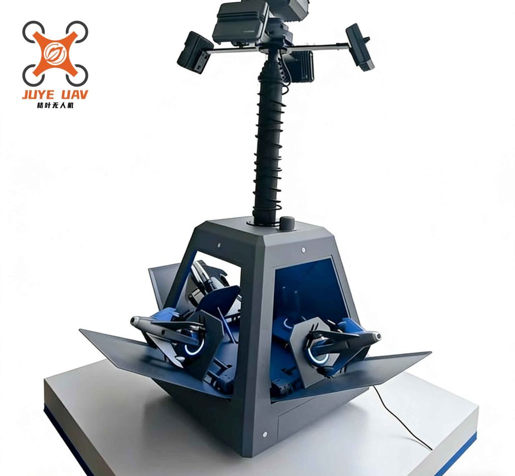
Globally, the urgency driven by recent conflicts has accelerated the development and deployment of acoustic anti-UAV systems. A comparative analysis of key international efforts reveals diverse approaches and architectural philosophies, summarized in the table below.
| Country/System | Key Features & Architecture | Reported Performance | Deployment & Cost |
|---|---|---|---|
| Ukraine (Distributed Network) | Large-scale distributed passive sonar network. Nodes consist of parabolic reflector, microphone, Android phone, battery. Uses AI/ML for classification and triangulation. | Range: ~5 km (UAV), ~7 km (cruise missile). Field of view: ~200°. False alarm rate: ~1.6%. | Mass deployment (reports of ~10,000 units). Rapid deployment (hours). Unit cost: ~$500 (lower in bulk). |
| Russia (Tactical Detector) | Compact unit with four microphones and processing/transmission unit. Fixed and portable versions. Continuous database updates. | Designed to detect UAVs regardless of RF frequency. Data via mobile network or radio (RS-485 interface). | Under testing. Designed for trenches, vehicles, and personal wear. |
| USA (Portable System) | Portable system focusing on acoustic signature detection and tracking (e.g., Raytheon’s D2TAS). | Range: 100-500+ m for multi-rotors. Provides azimuth, elevation, and track. | Deployed for tactical, portable anti-UAV operations. |
| Norway (Directional Array) | High-fidelity directional acoustic array (Discovair G2). 128 microphones + optical camera. Lightweight, low-power. | Provides “super-hearing,” target visualization, enhanced situational awareness. For extreme environments. | Used for specialized monitoring and perimeter security. |
| Denmark (Modular System) | Modular acoustic drone detector (Komodo). Can be used singly or in networked arrays. | Single unit: 250m radius, 360° coverage. Multi-unit networks cover >200,000 m². | Tested in NATO exercises (SET-348). Integrates with C2 systems. |
| Australia (Multi-Sensor Fusion) | Patented system combining radar and acoustic sensors (DroneShield). Radar cues acoustic analysis. | Reduces false alarms by distinguishing UAVs from clutter (birds, trees) before acoustic matching. | Emphasis on commercial and critical infrastructure protection. |
The operational principle of an advanced acoustic anti-UAV system can be mathematically described as a pipeline of signal processing stages. After the signal \( x_i(t) \) is acquired at each microphone \( i \) in an array, beamforming is often applied to enhance the signal from a specific direction \( \theta \). The output of a delay-and-sum beamformer is:
$$ y(t, \theta) = \sum_{i=1}^{M} w_i \cdot x_i(t – \Delta_i(\theta)) $$
where \( w_i \) are weighting coefficients and \( \Delta_i(\theta) \) are the steering delays aligned to direction \( \theta \). The power from this direction, \( P(\theta) = E[|y(t, \theta)|^2] \), is calculated to create an acoustic “image” or azimuth scan. For localization using TDOA with two sensors separated by distance \( d \), the bearing \( \phi \) relative to the array axis is given by:
$$ \phi = \arcsin\left(\frac{c \cdot \tau_{12}}{d}\right) $$
where \( c \) is the speed of sound (~343 m/s) and \( \tau_{12} \) is the estimated TDOA. In a distributed network with nodes at known positions \( \mathbf{p}_n = (x_n, y_n, z_n) \), the UAV position \( \mathbf{p}_u = (x_u, y_u, z_u) \) can be estimated by solving a set of hyperbolic equations derived from the TDOA measurements, often using nonlinear least-squares optimization:
$$ \min_{\mathbf{p}_u} \sum_{n>1} \left( \| \mathbf{p}_u – \mathbf{p}_n \| – \| \mathbf{p}_u – \mathbf{p}_1 \| – c \cdot \tau_{n1} \right)^2 $$
The heart of modern classification lies in feature extraction and AI. Common acoustic features include Mel-Frequency Cepstral Coefficients (MFCCs), spectral centroid, bandwidth, and zero-crossing rate. A simplified representation of an MFCC calculation involves: 1) Computing the power spectrum \( |X(f)|^2 \) via FFT, 2) Mapping to the Mel scale using a filterbank \( H_m(f) \), 3) Taking the logarithm, and 4) Applying the Discrete Cosine Transform (DCT):
$$ C_{\text{MFCC}}(k) = \sum_{m=1}^{M} \log \left( \sum_{f} |X(f)|^2 H_m(f) \right) \cdot \cos\left[ \frac{k(m-0.5)\pi}{M} \right] $$
These feature vectors \( \mathbf{C} \) are then fed into classifiers like Support Vector Machines (SVMs), Random Forests, or Deep Neural Networks (DNNs). A DNN model aims to learn a mapping \( f_{\text{DNN}}(\mathbf{C}) \) to a probability distribution over UAV classes \( \hat{y} \). The training minimizes a loss function \( \mathcal{L}(y, \hat{y}) \), such as cross-entropy, over a large dataset of labeled UAV and non-UAV sounds. The integration of AI is what transforms a simple noise detector into a reliable anti-UAV classification tool, significantly reducing false alarms caused by insects, birds, or ground vehicles.
Two dominant and interconnected trends are shaping the future of acoustic anti-UAV systems: Intelligentization and Networking. The Ukrainian network’s use of AI is a prime example of the first trend. As UAV designs evolve and background noise environments become more challenging, static database matching becomes insufficient. Adaptive machine learning algorithms that can learn new signatures in the field, perform few-shot learning, and leverage deep learning for robust feature extraction from raw audio are essential. Future systems will employ convolutional neural networks (CNNs) for spatial-spectral feature learning from array data and recurrent neural networks (RNNs) for temporal pattern analysis of engine harmonics. The performance metric for such an intelligent system can be framed as maximizing the F1-score, which balances precision (\( P \)) and recall (\( R \)):
$$ F1 = 2 \cdot \frac{P \cdot R}{P + R} = \frac{2 \cdot TP}{2 \cdot TP + FP + FN} $$
where \( TP, FP, FN \) are true positives, false positives, and false negatives, respectively. The goal of intelligentization is to push this score towards 1, even in low signal-to-noise ratio (SNR) conditions.
The second trend, networking, directly addresses the range limitation. By deploying a grid of low-cost acoustic nodes—inspired by the large-scale Ukrainian model—a wide-area acoustic surveillance blanket can be created. The effective detection radius \( R_{\text{network}} \) of a uniformly spaced grid with node spacing \( d \) is no longer the single-node range \( r \), but is extended by the grid’s coverage. For a square grid with \( N \) nodes covering an area \( A \), the relationship can be conceptually simplified as enabling persistent surveillance over \( A \), where \( A \approx N \cdot \pi r^2 \) for overlapping coverage. More importantly, networked nodes allow for more accurate and robust localization via multi-lateration and enable the fusion of heterogeneous data. A future anti-UAV network will integrate acoustic sensors with radar, RF detectors, and electro-optical/infrared (EO/IR) cameras. A Kalman filter or more advanced particle filter can be used to fuse these measurements. For a state vector \( \mathbf{x}_k \) (position, velocity) at time \( k \), the fusion process iterates between prediction and update:
$$ \begin{aligned}
\text{Prediction:} & \quad \hat{\mathbf{x}}_{k|k-1} = F_k \mathbf{x}_{k-1|k-1} \\
& \quad P_{k|k-1} = F_k P_{k-1|k-1} F_k^T + Q_k \\
\text{Update (with acoustic bearing \phi):} & \quad \tilde{y}_k = \phi_k – h(\hat{\mathbf{x}}_{k|k-1}) \\
& \quad S_k = H_k P_{k|k-1} H_k^T + R_k^{\text{acoustic}} \\
& \quad K_k = P_{k|k-1} H_k^T S_k^{-1} \\
& \quad \mathbf{x}_{k|k} = \hat{\mathbf{x}}_{k|k-1} + K_k \tilde{y}_k \\
& \quad P_{k|k} = (I – K_k H_k) P_{k|k-1}
\end{aligned} $$
Here, \( F_k \) is the state transition model, \( H_k \) is the observation model relating state to bearing, \( Q_k \) and \( R_k \) are process and measurement noise covariances, and \( K_k \) is the Kalman gain. This fused track is far more reliable than any single sensor could provide.
A particularly promising application of the networked, intelligent acoustic concept is in maritime and coastal defense. Acoustic sensor pods can be integrated into buoy systems, deployed on unmanned surface vessels (USVs), or attached to offshore platforms. The maritime environment, while having its own noise challenges (waves, ships), often has less persistent clutter than urban areas for low-altitude air targets. A network of maritime acoustic nodes could form a persistent picket line to detect anti-UAV threats approaching from the sea at very low altitudes, a zone notoriously difficult for ship-based radar due to sea clutter and the radar horizon limit. The detection range \( r_{\text{horizon}} \) for a radar at height \( h_{\text{radar}} \) to a target at height \( h_{\text{target}} \) is limited by the Earth’s curvature:
$$ r_{\text{horizon}} \approx \sqrt{2kR_e} \left( \sqrt{h_{\text{radar}}} + \sqrt{h_{\text{target}}} \right) $$
where \( R_e \) is Earth’s radius and \( k \) is the refraction factor. For a low-flying UAV (\( h_{\text{target}} \approx 10 \)m) and a ship’s radar at 30m, this range is only about 25-30 km. Distributed acoustic sensors on floating platforms can help fill this gap closer to the threat axis, cueing other sensors and weapons systems. The logistical and cost equation for such a maritime acoustic layer is favorable compared to deploying additional high-power radar systems.
In conclusion, acoustic detection represents a vital, evolving, and cost-effective strand in the broader anti-UAV defense matrix. Its passivity, low cost, and effectiveness against low-RF-signature targets ensure its place in both military and critical infrastructure protection schemes. The future of this technology lies not in attempting to make it a long-range, standalone solution, but in fully embracing its strengths within a networked, multi-sensor architecture. By leveraging advances in AI for robust classification and adaptive learning, and by deploying large-scale, distributed networks of intelligent acoustic nodes—especially in hard-to-cover domains like complex terrain, urban canyons, and the maritime approaches—acoustic systems will significantly enhance the resilience and effectiveness of integrated anti-UAV systems. The ongoing global research and real-world deployment of these systems provide a clear roadmap: the path forward is one of convergence, where simple acoustic sensors become intelligent nodes in a vast, collaborative sensing web dedicated to countering the ever-evolving UAV threat.