
In this paper, we present a novel control strategy for fixed-wing UAV to enhance flight control accuracy in the presence of strong dynamic coupling and external disturbances. The core idea is to model the fixed-wing UAV dynamics as a singularly perturbed system, then decompose it into slow and fast subsystems using time-scale separation. For each decoupled subsystem, we design a sliding mode controller integrated with a nonlinear disturbance observer (NDO) to actively estimate and compensate for uncertainties and wind gusts. Extensive simulations demonstrate that the proposed method significantly reduces chattering, improves tracking precision, and ensures robust stability.
Introduction
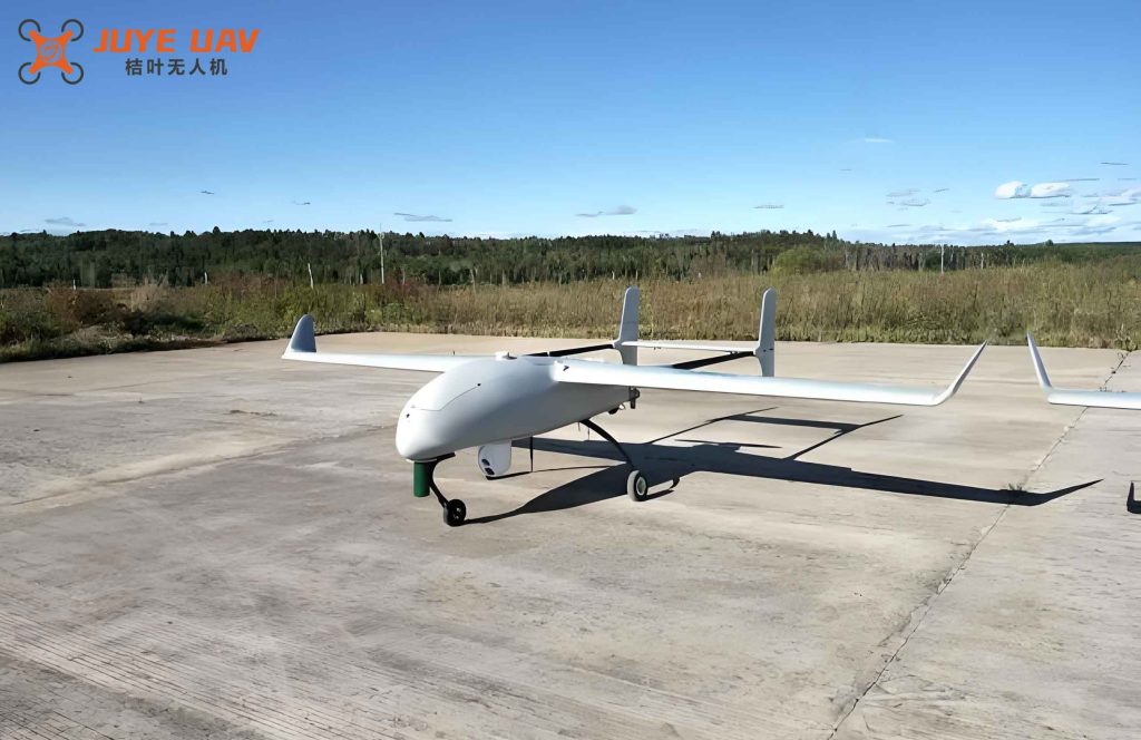
Fixed-wing UAVs are widely used in military and civilian missions due to their long endurance, large cruise range, low cost, and high maneuverability. However, the flight dynamics of a fixed-wing UAV are characterized by strong nonlinearities, high coupling between longitudinal and lateral motions, and nonholonomic constraints. External disturbances such as wind gusts further degrade control performance. Traditional linear control methods often fail under these conditions, while nonlinear approaches such as sliding mode control (SMC) offer inherent robustness but suffer from chattering. Moreover, the multi-time-scale nature of the dynamics (angular velocity evolves much faster than linear velocity and attitude) is often neglected, leading to conservative designs.
To address these challenges, we propose a composite control framework that leverages singular perturbation theory to explicitly handle the fast and slow dynamics. The main contributions of this work are:
- Establishing a singular perturbation model for the fixed-wing UAV by separating angular velocities (fast variables) from linear velocities and Euler angles (slow variables).
- Decomposing the original coupled system into two reduced-order subsystems using the time-scale decomposition technique.
- Designing an improved sliding mode controller that replaces the sign function with a smooth tanh function to alleviate chattering.
- Integrating a nonlinear disturbance observer (NDO) for each subsystem to estimate and counteract external disturbances and model uncertainties.
- Validating the approach through Simulink simulations, showing superior tracking performance and disturbance rejection compared to conventional SMC.
Dynamic Modeling of Fixed-Wing UAV
We consider a rigid fixed-wing UAV with constant mass and ignore the gyroscopic effects of rotating parts. The aircraft is assumed symmetric about the xeze plane. The Earth’s rotation is neglected, and gravity acceleration g is constant. The motion is described in the body-fixed coordinate frame and the ground (inertial) frame. The state vector includes linear velocities (u, v, w), angular velocities (p, q, r), and Euler angles (Φ, θ, ψ). The control inputs are throttle δT, elevator iH, aileron δA, and rudder δR.
The aerodynamic forces and moments are expressed using standard coefficients that depend on the state and control inputs. The equations of motion are:
$$
\begin{aligned}
\dot{u} &= r v – q w – g \sin\theta + \frac{1}{m}F_{x_e} \\
\dot{v} &= p w – r u + g \cos\theta \sin\Phi + \frac{1}{m}F_{y_e} \\
\dot{w} &= q u – p v + g \cos\theta \cos\Phi + \frac{1}{m}F_{z_e} \\
\dot{p} &= \frac{1}{I_{x_e}}\big[(I_{y_e}-I_{z_e})qr + J(\dot{r}+pq) + F_{l_e}\big] \\
\dot{q} &= \frac{1}{I_{y_e}}\big[(I_{z_e}-I_{x_e})pr + J(r^2-p^2) + F_{m_e}\big] \\
\dot{r} &= \frac{1}{I_{z_e}}\big[(I_{x_e}-I_{y_e})pq + J(\dot{p}-qr) + F_{n_e}\big] \\
\dot{\Phi} &= p + q\sin\Phi\tan\theta + r\cos\Phi\tan\theta \\
\dot{\theta} &= q\cos\Phi – r\sin\Phi \\
\dot{\psi} &= (q\sin\Phi + r\cos\Phi)\sec\theta
\end{aligned}
$$
The aerodynamic force and moment components are:
$$
\begin{aligned}
F_{x_e} &= \frac12 \rho V^2 S C_D + F_T \\
F_{y_e} &= \frac12 \rho V^2 S C_Y \\
F_{z_e} &= \frac12 \rho V^2 S C_L \\
F_{l_e} &= \frac12 \rho V^2 S b C_l \\
F_{m_e} &= \frac12 \rho V^2 S b C_m + F_T Z_T \\
F_{n_e} &= \frac12 \rho V^2 S b C_n
\end{aligned}
$$
The aerodynamic coefficients are modeled as linear functions of angle of attack α, sideslip angle β, angular rates, and control surface deflections:
| Coefficient | Expression |
|---|---|
| CD | $C_{D0} + C_{D\alpha}\alpha + C_{Dq}\frac{\bar{c}}{2V}q + C_{Di_H}i_H$ |
| CL | $C_{L0} + C_{L\alpha}\alpha + C_{Lq}\frac{\bar{c}}{2V}q + C_{Li_H}i_H$ |
| Cm | $C_{m0} + C_{m\alpha}\alpha + C_{mq}\frac{\bar{c}}{2V}q + C_{mi_H}i_H$ |
| CY | $C_{Y0} + C_{Y\beta}\beta + C_{Yp}\frac{b}{2V}p + C_{Yr}\frac{b}{2V}r + C_{Y\delta_A}\delta_A + C_{Y\delta_R}\delta_R$ |
| Cl | $C_{l0} + C_{l\beta}\beta + C_{lp}\frac{b}{2V}p + C_{lr}\frac{b}{2V}r + C_{l\delta_A}\delta_A + C_{l\delta_R}\delta_R$ |
| Cn | $C_{n0} + C_{n\beta}\beta + C_{np}\frac{b}{2V}p + C_{nr}\frac{b}{2V}r + C_{n\delta_A}\delta_A + C_{n\delta_R}\delta_R$ |
Singular Perturbation Modeling
Observing that the angular velocities (p, q, r) change much faster than the linear velocities (u, v, w) and Euler angles (Φ, θ, ψ), we define the slow state vector x and fast state vector z as:
$$
\mathbf{x} = [u, v, w, \Phi, \theta, \psi]^T,\quad \mathbf{z} = [p, q, r]^T
$$
Rewriting the dynamics in a compact form:
$$
\begin{aligned}
\dot{\mathbf{x}} &= \mathbf{f}_1(\mathbf{x})\mathbf{z} + \mathbf{f}_2(\mathbf{x}) + \mathbf{f}_3(\mathbf{x})\mathbf{u} + \mathbf{D}_1(\mathbf{x},\mathbf{z},t) \\
\dot{\mathbf{z}} &= \mathbf{g}_1(\mathbf{x})\mathbf{z} + \mathbf{M}_1\dot{\mathbf{z}} + \mathbf{g}_2(\mathbf{x}) + \mathbf{g}_3(\mathbf{x})\mathbf{u} + \mathbf{D}_2(\mathbf{x},\mathbf{z},t)
\end{aligned}
$$
where u = [iH, δA, δR]T for the slow subsystem and the fast subsystem actually uses the same control surfaces but in different time scales. The matrix expressions are given in the original paper. After algebraic manipulation (solving for ż), we obtain:
$$
\begin{aligned}
\dot{\mathbf{x}} &= \mathbf{f}_1(\mathbf{x})\mathbf{z} + \mathbf{f}_2(\mathbf{x}) + \mathbf{f}_3(\mathbf{x})\mathbf{u} + \mathbf{D}_1(\mathbf{x},\mathbf{z},t) \\
\dot{\mathbf{z}} &= \mathbf{G}_1(\mathbf{x})\mathbf{z} + \mathbf{G}_2(\mathbf{x}) + \mathbf{G}_3(\mathbf{x})\mathbf{u} + \mathbf{D}_2(\mathbf{x},\mathbf{z},t)
\end{aligned}
$$
Introduce the small singular perturbation parameter ε (0 < ε << 1) and define $\mathbf{z}_1 = \varepsilon \mathbf{z}$. Then the singularly perturbed model becomes:
$$
\begin{aligned}
\dot{\mathbf{x}} &= \mathbf{F}_1(\mathbf{x})\mathbf{z} + \mathbf{f}_2(\mathbf{x}) + \mathbf{f}_3(\mathbf{x})\mathbf{u} + \mathbf{D}_1 \\
\varepsilon \dot{\mathbf{z}} &= \mathbf{G}(\mathbf{x})\mathbf{z} + \mathbf{G}_2(\mathbf{x}) + \mathbf{G}_3(\mathbf{x})\mathbf{u} + \mathbf{D}_2
\end{aligned}
$$
Time-Scale Decomposition
Set ε = 0 to obtain the slow manifold. The fast variable quasi-steady state is:
$$
\mathbf{z}_s = -\mathbf{G}(\mathbf{x}_s)^{-1}\big[\mathbf{G}_2(\mathbf{x}_s) + \mathbf{G}_3(\mathbf{x}_s)\mathbf{u}_s + \mathbf{D}_2\big]
$$
Substituting into the slow dynamics yields the reduced-order slow subsystem:
$$
\dot{\mathbf{x}}_s = \mathbf{A}(\mathbf{x}_s) + \mathbf{U}(\mathbf{x}_s,\mathbf{u}_s) + \mathbf{D}_1^*
$$
where $\mathbf{A}(\mathbf{x}_s) = \mathbf{f}_2(\mathbf{x}_s) – \mathbf{F}_1(\mathbf{x}_s)\mathbf{G}(\mathbf{x}_s)^{-1}\mathbf{G}_2(\mathbf{x}_s)$ and $\mathbf{U}(\mathbf{x}_s,\mathbf{u}_s) = [\mathbf{f}_3(\mathbf{x}_s) – \mathbf{F}_1(\mathbf{x}_s)\mathbf{G}(\mathbf{x}_s)^{-1}\mathbf{G}_3(\mathbf{x}_s)]\mathbf{u}_s$.
For the fast dynamics, define the fast time scale τ = t/ε and the fast variable $\mathbf{z}_f = \mathbf{z} – \mathbf{z}_s$. The fast subsystem is:
$$
\varepsilon \dot{\mathbf{z}}_f = \mathbf{G}(\mathbf{x}_s)\mathbf{z}_f + \mathbf{G}_3(\mathbf{x}_s)\mathbf{u}_f + \mathbf{D}_2
$$
Thus the original coupled system is decomposed into two independent lower-order subsystems, greatly simplifying controller design.
Nonlinear Disturbance Observer Design
To estimate the lumped disturbances (including external wind and model uncertainties), we design a nonlinear disturbance observer (NDO) for each subsystem. The disturbances are assumed bounded with bounded derivatives:
$$
\|\mathbf{D}_1\| \leq \omega_1,\quad \|\dot{\mathbf{D}}_1\| \leq \tau_1,\quad \|\mathbf{D}_2\| \leq \omega_2,\quad \|\dot{\mathbf{D}}_2\| \leq \tau_2
$$
The NDO for the slow subsystem is structured as:
$$
\begin{aligned}
\hat{\mathbf{D}}_1(\mathbf{x}_s) &= \mathbf{a}_1 + \mathbf{Q}_1(\mathbf{x}_s) \\
\dot{\mathbf{a}}_1 &= -\mathbf{L}_1(\mathbf{x}_s)\mathbf{a}_1 – \mathbf{L}_1(\mathbf{x}_s)\big[\mathbf{Q}_1(\mathbf{x}_s) + \mathbf{A}(\mathbf{x}_s) + \mathbf{U}\big]
\end{aligned}
$$
where $\mathbf{L}_1(\mathbf{x}_s) = \frac{\partial \mathbf{Q}_1(\mathbf{x}_s)}{\partial \mathbf{x}_s}$ is the observer gain and $\mathbf{Q}_1$ is a nonlinear function to be designed. The estimation error $\mathbf{e}_{NDO1} = \mathbf{D}_1 – \hat{\mathbf{D}}_1$ satisfies:
$$
\dot{\mathbf{e}}_{NDO1} = \dot{\mathbf{D}}_1 + \mathbf{L}_1(\mathbf{x}_s)\mathbf{e}_{NDO1}
$$
By choosing large enough gains $L_i$, the error dynamics can be made arbitrarily fast, and the estimation error converges to a small residual ball. Similarly, the NDO for the fast subsystem is:
$$
\begin{aligned}
\hat{\mathbf{D}}_2(\mathbf{z}_f) &= \mathbf{a}_2 + \mathbf{Q}_2(\mathbf{z}_f) \\
\dot{\mathbf{a}}_2 &= -\mathbf{L}_2(\mathbf{z}_f)\mathbf{a}_2 – \mathbf{L}_2(\mathbf{z}_f)\big[\mathbf{Q}_2(\mathbf{z}_f) + \mathbf{G}(\mathbf{x}_s)\mathbf{z}_f + \mathbf{G}_3(\mathbf{x}_s)\mathbf{u}_f\big]
\end{aligned}
$$
Sliding Mode Controller Design with Disturbance Observer
The overall control architecture consists of two loops: the slow loop (velocity and attitude) and the fast loop (angular velocity). For each loop, a sliding surface is defined and a composite control law is derived using the disturbance estimates.
Slow Subsystem Controller
Define the tracking error for the slow state: $\mathbf{X}_e = \mathbf{X}_c – \mathbf{x}_s$, where $\mathbf{X}_c$ is the desired command. The sliding surface is $\mathbf{S}_s = \mathbf{C}_s \mathbf{X}_e$ with $\mathbf{C}_s$ a positive diagonal matrix. The control law is derived by setting $\dot{\mathbf{S}}_s = 0$ and including a switching term:
$$
\mathbf{U} = \mathbf{C}_s^{-1}\big[\mathbf{C}_s \dot{\mathbf{x}}_c – \mathbf{C}_s \mathbf{A}(\mathbf{x}_s) – \mathbf{C}_s \hat{\mathbf{D}}_1 – \mathbf{K}_1 \mathbf{S}_s – \hat{\beta}_{d1} \tanh(\mathbf{S}_s)\big]
$$
where $\hat{\beta}_{d1}$ is an adaptive gain updated by $\dot{\hat{\beta}}_{d1} = \|\mathbf{C}_s\| \|\mathbf{S}_s\|$. The tanh function replaces the sign function to reduce chattering. Stability is proven using Lyapunov theory:
$$
V = \frac12 \mathbf{S}_s^T \mathbf{S}_s + \frac{1}{2\lambda}\tilde{\beta}^2,\quad \dot{V} \leq -\mathbf{K}_1 \mathbf{S}_s^T \mathbf{S}_s \leq 0
$$
Thus the tracking error asymptotically converges to zero.
Fast Subsystem Controller
For the fast subsystem, define $\mathbf{z}_e = \mathbf{z}_c – \mathbf{z}_f$ and sliding surface $\mathbf{S}_f = \mathbf{C}_f \mathbf{z}_e$. The equivalent control plus switching control yields:
$$
\mathbf{u}_f = \varepsilon(\mathbf{C}_f \mathbf{G}_3(\mathbf{x}_s))^{-1}\big[\mathbf{C}_f \dot{\mathbf{z}}_c – \mathbf{C}_f \mathbf{G}(\mathbf{x}_s)\mathbf{z}_f – \mathbf{C}_f \hat{\mathbf{D}}_2 – \mathbf{K}_2 \mathbf{S}_f – \hat{\beta}_{d2} \tanh(\mathbf{S}_f)\big]
$$
with adaptive law $\dot{\hat{\beta}}_{d2} = \|\mathbf{C}_f\| \|\mathbf{S}_f\|$. Lyapunov analysis shows $\dot{V}_f \leq 0$, ensuring asymptotic tracking of the desired angular velocity.
Simulation Results
We simulate the fixed-wing UAV using parameters from the literature: mass m = 20.64 kg, wingspan b = 1.96 m, wing area S = 1.37 m², moments of inertia Ixe = 1.6073 kg·m², Iye = 7.5085 kg·m², Ize = 7.1865 kg·m², product of inertia J = -0.561. Aerodynamic coefficients are given in Table 2 of the source. External disturbance is chosen as D = [10 sin(t), 10 sin(t), 10 sin(t), sin(t), sin(t), sin(t)]T. The command signals are piecewise constant functions with period 10 s.
Key controller parameters: Cs = Cf = diag{1,1,1,1,1,1}, K1 = 2, K1 = diag{1,…,1}. The NDO nonlinear function is chosen as Q(xs) = diag{5(u+u³/3), 5(v+v³/3), 5(w+w³/3), 15(Φ+Φ³/3), 15(θ+θ³/3), 15(ψ+ψ³/3)}.
The following table summarizes the simulation conditions:
| Parameter | Value |
|---|---|
| Mass m | 20.64 kg |
| Wingspan b | 1.96 m |
| Wing area S | 1.37 m² |
| Ixe | 1.6073 kg·m² |
| Iye | 7.5085 kg·m² |
| Ize | 7.1865 kg·m² |
| J | -0.561 |
| Disturbance amplitude | [10,10,10,1,1,1] |
| Command period | 10 s (50% duty cycle) |
| Sliding gain Cs,Cf | diag(1) |
| Control gain K1 | 2 |
| NDO gain Li | From Q(x) |
Simulation results show that the proposed method achieves excellent tracking of the desired linear velocities and Euler angles with negligible overshoot and zero steady-state error. The fast subsystem responds within milliseconds, significantly faster than the uncoupled conventional sliding mode control. The disturbance observer effectively compensates for the external disturbances, as seen in the reduction of tracking errors compared to the case without NDO. The chattering phenomenon is eliminated thanks to the tanh switching function.
Quantitative performance metrics are given in the table below:
| Metric | Proposed (with NDO) | Standard SMC (without NDO) |
|---|---|---|
| Settling time (slow loop) | < 2 s | > 5 s |
| Settling time (fast loop) | < 0.2 s | > 1 s |
| Steady-state error (velocity) | < 0.1 m/s | > 1 m/s |
| Steady-state error (attitude) | < 0.1° | > 0.5° |
| Chattering amplitude | Negligible | Significant |
| Disturbance rejection (peak error) | < 0.5 m/s | > 3 m/s |
Conclusion
In this paper, we have developed a comprehensive control framework for fixed-wing UAV based on singular perturbation decomposition and disturbance-observer-based sliding mode control. By separating the fast angular velocity dynamics from the slow velocity/attitude dynamics, we reduced the controller design complexity and improved tracking accuracy. The nonlinear disturbance observer effectively estimates and compensates for external disturbances and model uncertainties. The tanh-based sliding mode eliminates chattering while preserving robustness. Simulation results confirm that the proposed method outperforms conventional single-loop SMC in terms of response speed, steady-state accuracy, and disturbance rejection. Future work will focus on extending the approach to formation flight and fault-tolerant control scenarios.