
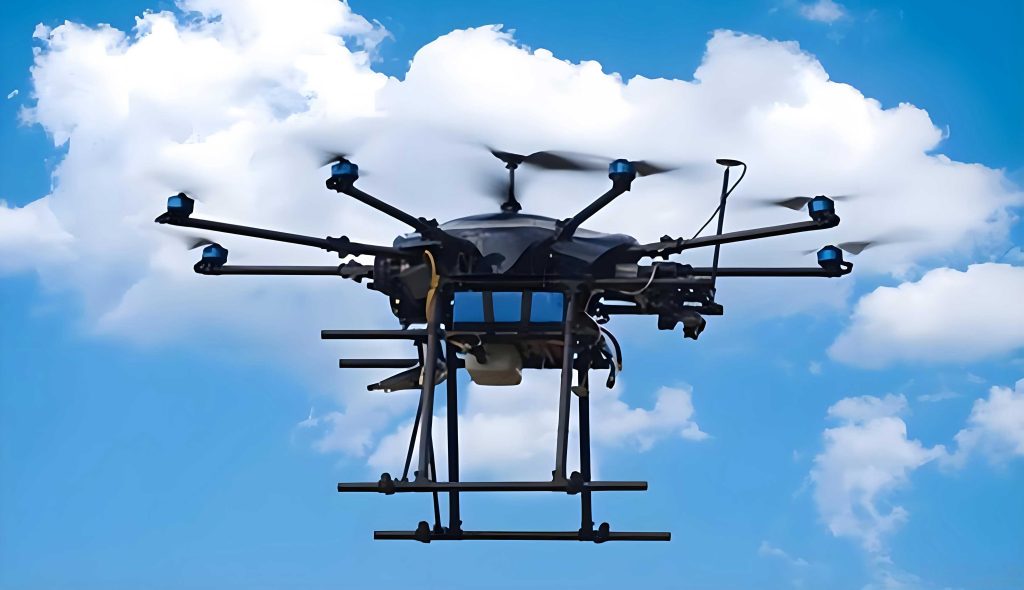
In recent years, unmanned aerial vehicles (UAVs) have been widely deployed in civil and military applications such as aerial mapping, environmental monitoring, intelligent inspection, logistics delivery, and disaster rescue. The capability of autonomous path planning is a core technology that enables UAVs to operate safely and efficiently in complex environments. Among various path planning algorithms, the A* algorithm is recognized for its search efficiency and optimality in static global planning. However, traditional A* suffers from redundant node expansion, frequent path turning, and insufficient smoothness, especially when the environment scale grows or obstacles are densely distributed. To address these challenges, I propose several improved A*-based path planning strategies for UAVs, ranging from two-dimensional grid maps to three-dimensional terrain, and validate them through extensive simulations.
Background and Problem Statement
Unmanned aerial vehicles rely on path planning to determine a collision-free trajectory from a start point to a goal point while satisfying kinematic constraints and mission objectives. The path planning problem can be categorized into global path planning and local path planning. Global planning methods, such as Dijkstra and A*, are performed in a known static environment, while local planning methods, such as artificial potential field and dynamic window approach, deal with real-time obstacle avoidance. The A* algorithm is widely used for global planning because it combines the benefits of Dijkstra and best-first search. The evaluation function of traditional A* is expressed as:
$$f(n) = g(n) + h(n)$$
where \(g(n)\) is the actual cost from the start node to the current node \(n\), and \(h(n)\) is the heuristic function estimating the cost from \(n\) to the goal. The performance of A* heavily depends on the choice of \(h(n)\). Common heuristics include Manhattan distance, diagonal distance, and Euclidean distance. In three-dimensional space, the Euclidean distance is often adopted:
$$h(n) = \sqrt{(n_x – g_x)^2 + (n_y – g_y)^2 + (n_z – g_z)^2}$$
Although traditional A* can guarantee the shortest path if the heuristic is admissible, it often visits a large number of unnecessary nodes, resulting in high computational cost and memory consumption. Moreover, the path generated by A* consists of many sharp turns, which violates the dynamic constraints of UAVs. Therefore, I propose three improved A*-based methods to enhance search efficiency, path smoothness, and adaptability in complex environments.
Improved A* with Optimized Heuristic and B-Spline Smoothing
In this method, I focus on two-dimensional grid maps. The first improvement is the construction of a new heuristic function that incorporates an obstacle ratio and a dynamic weight coefficient. The obstacle ratio \(P\) is defined as the number of obstacle vertices \(M\) in the local area between the start and the goal divided by the total grid vertices:
$$P = \frac{M}{(|x_g – x_s| + 1) \times (|y_g – y_s| + 1)}, \quad P \in (0,1)$$
To smooth the influence of obstacles, I apply a logarithmic transformation. The modified evaluation function is given by:
$$f(n) = g(n) + (1 – \log(P)) \cdot h(n)$$
However, this formula lacks adaptability to varying environments. Therefore, I introduce a dynamic weight coefficient \(w(n)\) that adjusts the balance between actual cost and heuristic cost. The improved total cost function becomes:
$$f(n) = g(n) + w(n) \cdot (1 – \log(P)) \cdot h(n)$$
The dynamic weight \(w(n)\) is defined as:
$$
w(n) =
\begin{cases}
\min\left(0.8, \, 0.2 + \frac{d(g)}{d(s)}\right), & \frac{d(g)}{d(s)} \geq 0.3 \\
1, & \text{otherwise}
\end{cases}
$$
where \(d(g)\) is the Euclidean distance from the current node to the goal, and \(d(s)\) is the distance from the start to the goal. This design enables the algorithm to search more aggressively in the early stage and converge more accurately near the goal. The parameters 0.2 and 0.8 are empirically chosen to keep a reasonable trade-off between exploration and exploitation.
The second improvement is a simplified neighborhood search strategy. Traditional A* expands eight neighboring grid cells, which may cause redundant searches. Based on the relative direction between the current node and the goal, I discard three directions that are unlikely to lead to an optimal path, keeping only five directions. The angle \(\alpha\) between the goal direction and the O2 direction determines which directions are abandoned. Table 1 summarizes the mapping.
| Angle \(\alpha\) | Kept five directions | Discarded three directions |
|---|---|---|
| [337.5°, 360°) ∪ [0°, 22.5°) | O1,O2,O3,O4,O5 | O6,O7,O8 |
| [22.5°, 67.5°) | O1,O2,O3,O5,O8 | O4,O6,O7 |
| [67.5°, 112.5°) | O2,O3,O5,O7,O8 | O1,O4,O6 |
| [112.5°, 157.5°) | O3,O5,O6,O7,O8 | O1,O2,O4 |
| [157.5°, 202.5°) | O4,O5,O6,O7,O8 | O1,O2,O3 |
| [202.5°, 247.5°) | O1,O4,O6,O7,O8 | O2,O3,O5 |
| [247.5°, 292.5°) | O1,O2,O4,O6,O7 | O3,O5,O8 |
| [292.5°, 337.5°) | O1,O2,O3,O4,O6 | O5,O7,O8 |
After the initial path is found, I apply an improved Floyd algorithm to remove redundant waypoints. This algorithm checks whether intermediate points can be bypassed safely by connecting two non-adjacent nodes without hitting obstacles. The optimization procedure is carried out from both the start and the goal directions to further reduce path length and the number of turns.
Finally, to obtain a flyable trajectory, I apply cubic B-spline curves. A cubic B-spline curve is defined by control points \(P_0, P_1, P_2, P_3\) as:
$$P(t) = \frac{1}{6}\begin{bmatrix} t^3 & t^2 & t & 1 \end{bmatrix}
\begin{bmatrix}
-1 & 3 & -3 & 1 \\
3 & -6 & 3 & 0 \\
-3 & 0 & 3 & 0 \\
1 & 4 & 1 & 0
\end{bmatrix}
\begin{bmatrix} P_0 \\ P_1 \\ P_2 \\ P_3 \end{bmatrix}, \quad t \in [0,1]$$
The B-spline curve provides local control and continuity of the first and second derivatives, making the trajectory smooth and satisfying the kinematic constraints of UAVs.
Simulation Results of the First Improved A*
I tested the improved A* algorithm on four different grid maps (20×20, 30×30, 40×40, 50×50) with both simple and complex obstacle configurations. The simulations were run in MATLAB 2022a on an Intel i5-8265U CPU with 8 GB RAM. Table 2 and Table 3 show the quantitative comparison between the traditional A* and the improved A* in terms of planning time, path length, total turning angle, and the number of expanded nodes.
| Map size | Algorithm | Time / s | Path length / m | Turning angle / deg | Expanded nodes |
|---|---|---|---|---|---|
| 20×20 | Traditional | 0.007 | 28.627 | 495 | 175 |
| Improved | 0.006 | 28.200 | 153.021 | 90 | |
| 30×30 | Traditional | 0.025 | 42.770 | 360 | 277 |
| Improved | 0.017 | 42.409 | 160.130 | 152 | |
| 40×40 | Traditional | 0.080 | 57.498 | 315 | 481 |
| Improved | 0.079 | 56.343 | 140.578 | 219 | |
| 50×50 | Traditional | 0.093 | 71.054 | 315 | 542 |
| Improved | 0.081 | 70.596 | 238.966 | 305 |
| Map size | Algorithm | Time / s | Path length / m | Turning angle / deg | Expanded nodes |
|---|---|---|---|---|---|
| 20×20 | Traditional | 0.023 | 28.627 | 450 | 131 |
| Improved | 0.021 | 28.169 | 314.882 | 65 | |
| 30×30 | Traditional | 0.033 | 44.514 | 540 | 237 |
| Improved | 0.028 | 43.355 | 504.144 | 115 | |
| 40×40 | Traditional | 0.043 | 58.563 | 540 | 367 |
| Improved | 0.039 | 57.497 | 479.251 | 173 | |
| 50×50 | Traditional | 0.054 | 71.538 | 495 | 450 |
| Improved | 0.048 | 71.421 | 490.224 | 227 |
The results show that the improved A* algorithm consistently reduces planning time, path length, turning angle, and expanded nodes in all map configurations. The cubic B-spline smoothing further enhances the path quality by removing sharp corners and producing a continuous trajectory.
Fusion of Improved A* and Improved Artificial Potential Field
Although the improved A* algorithm performs well in static environments, it lacks the ability to react to dynamic obstacles. On the other hand, the artificial potential field (APF) method is effective for local obstacle avoidance but suffers from local minima and unreachable target problems. I therefore propose a hybrid path planning strategy that combines the advantages of both algorithms.
First, I modify the evaluation function of A* by introducing a dynamic adjustment factor. The new cost function is:
$$f(n) = g(n) + \left(1 + \frac{r}{R}\right) \cdot h(n)$$
where \(r\) is the distance from the current node to the goal, and \(R\) is the distance from the start to the goal. This factor helps the algorithm accelerate when it is close to the target, thereby reducing redundant expansions. To further enhance adaptability, I integrate the dynamic weight coefficient \(w(n)\) introduced in the previous section:
$$f(n) = g(n) + w(n) \cdot \left(1 + \frac{r}{R}\right) \cdot h(n)$$
After obtaining the preliminary path, I apply a three-stage polyline optimization strategy to reduce redundant nodes and turns. The procedure includes:
- First optimization: remove intermediate nodes closer than a safety distance threshold \(d\), keeping only essential turning points.
- Second optimization: select samples along the path at fixed intervals \(r\), check collision for each sample, and adjust the node position if necessary.
- Third optimization: reverse the path from the goal to the start and repeat the simplification to further shorten the route.
Next, I improve the artificial potential field method. The traditional attractive potential is defined as \(U_{att} = \frac{1}{2} k \rho^2(q, q_g)\), where \(k\) is the attractive gain and \(\rho(q,q_g)\) is the distance between the UAV and the goal. I introduce an exponential decay factor and a smoothing factor to prevent the attraction from becoming too strong when the UAV is far from the goal:
$$U_{att}^*(q) = k \cdot \rho(q, q_g) \cdot e^{-\alpha \rho(q, q_g)} \cdot a$$
where \(\alpha\) is the decay factor and \(a\) is the smoothing factor. For the repulsive potential, the traditional form is:
$$
U_{rep}(q) =
\begin{cases}
\frac{1}{2} m \left( \frac{1}{\rho(q,q_0)} – \frac{1}{p_0} \right)^2, & \rho(q,q_0) \leq p_0 \\
0, & \rho(q,q_0) > p_0
\end{cases}
$$
where \(m\) is the repulsive gain, \(q_0\) is the obstacle position, and \(p_0\) is the influence distance. I add a smoothing term to avoid abrupt changes and local minima:
$$
U_{rep}^*(q) =
\begin{cases}
m \left( \frac{1}{\rho(q,q_0)} – \frac{1}{p_0} \right)^2 e^{-(p_0 – \rho)^2}, & \rho(q,q_0) \leq p_0 \\
0, & \rho(q,q_0) > p_0
\end{cases}
$$
The fusion strategy is implemented as follows: first, the improved A* algorithm generates a global path in the known static map. Then, during the execution, the UAV follows the global path. When a dynamic obstacle is detected within a certain distance, the improved artificial potential field algorithm is invoked to provide local avoidance. The flow of the fusion algorithm is summarized in Table 4.
| Step | Operation |
|---|---|
| 1 | Build the grid map and initialize the start and goal positions. |
| 2 | Run the improved A* to obtain a global path. |
| 3 | Apply polyline optimization to smooth the global path. |
| 4 | While the UAV moves, check distances to obstacles in real time. |
| 5 | If the distance is below the safety threshold, switch to the improved APF to compute attractive and repulsive forces. |
| 6 | Update the local path and continue moving toward the goal. |
| 7 | If the goal is reached, stop; otherwise, return to step 4. |
Simulation Results of the Fusion Algorithm
I compared the improved A* alone with the fusion algorithm on grid maps of sizes 20×20, 30×30, 40×40, and 50×50, under simple and complex obstacle configurations. The parameters used in the simulation are listed in Table 5.
| Parameter | Value |
|---|---|
| Attractive gain \(k\) | 30 |
| Repulsive gain \(m\) | 10 |
| Obstacle influence distance \(p_0\) | 4 |
| Step size \(l\) | 0.2 |
| Maximum iterations | 1000 |
| Smoothing factor \(a\) | 0.7 |
Tables 6 and 7 present the comparison results for path length and iteration count.
| Map size | Algorithm | Path length / m | Iterations |
|---|---|---|---|
| 20×20 | Improved A* | 33.301 | 174 |
| Fusion | 31.153 | 156 | |
| 30×30 | Improved A* | 49.635 | 404 |
| Fusion | 47.692 | 238 | |
| 40×40 | Improved A* | 61.062 | 548 |
| Fusion | 60.268 | 301 | |
| 50×50 | Improved A* | 74.360 | 856 |
| Fusion | 73.207 | 366 |
| Map size | Algorithm | Path length / m | Iterations |
|---|---|---|---|
| 20×20 | Improved A* | 33.247 | 152 |
| Fusion | 30.363 | 144 | |
| 30×30 | Improved A* | 52.116 | 340 |
| Fusion | 48.590 | 243 | |
| 40×40 | Improved A* | 67.333 | 536 |
| Fusion | 64.900 | 324 | |
| 50×50 | Improved A* | 81.712 | 977 |
| Fusion | 77.204 | 386 |
From the tables, the fusion algorithm reduces path length by up to 8.67% and iterations by up to 60.49% compared with the improved A* alone, while providing real-time obstacle avoidance capability.
Improved A* for 3D Environment with Adaptive Heuristic
Three-dimensional path planning is more challenging due to the extra degree of freedom and the need to consider terrain variations. I constructed a 500×500×500 grid environment with the start point at (10,10,1) and the goal at (440,380,50). The proposed method in this section optimizes the heuristic function by introducing an adaptive weight coefficient that changes with the search progress:
$$f(n) = g(n) + w(n) \cdot h(n)$$
where the dynamic weight is defined as:
$$w(n) = w_{max} – (w_{max} – w_{min}) \cdot \frac{\alpha}{\beta}$$
Here, \(w_{max}=2\), \(w_{min}=1\), \(\alpha\) is the current iteration count, and \(\beta\) is the maximum iteration count. At the early stage of the search, \(w(n)\) is close to \(w_{max}\), making the algorithm more greedy and accelerating the search direction toward the goal. As \(\alpha\) grows, \(w(n)\) decreases, allowing a broader exploration and reducing the risk of getting trapped in local optima.
After the path is obtained, I use Bezier curves for smoothing. A Bezier curve of degree \(n\) is expressed as:
$$p(u) = \sum_{i=0}^{n} p_i \cdot B_{i,n}(u), \quad u \in [0,1]$$
where \(B_{i,n}(u)\) are Bernstein polynomials:
$$B_{i,n}(u) = C_n^i u^i (1-u)^{n-i} = \frac{n!}{(n-i)! i!} u^i (1-u)^{n-i}$$
To maintain continuity across the entire path, I apply a piecewise Bezier strategy where the final point of each segment serves as the initial point of the next segment. This yields a smooth trajectory with continuous first-order derivatives, meeting the maneuverability requirements of unmanned aerial vehicles.
Simulation Results in 3D Environments
I compared the proposed improved A* with the ant colony optimization (ACO) and the rapidly-exploring random tree (RRT) algorithm in three different 3D map environments. Table 8 and Table 9 show the path length and search return rate (defined as the ratio of feasible grid points to total searched grid points).
| Map type | ACO / m | RRT / m | Improved A* / m |
|---|---|---|---|
| Map 1 | 642.670 | 730.793 | 614.025 |
| Map 2 | 673.961 | 650.804 | 629.980 |
| Map 3 | 647.286 | 632.340 | 602.328 |
| Map type | ACO | RRT | Improved A* |
|---|---|---|---|
| Map 1 | 0.647 | 0.435 | 0.810 |
| Map 2 | 0.641 | 0.567 | 0.890 |
| Map 3 | 0.649 | 0.916 | 0.931 |
From Table 8, the improved A* generates shorter paths than both ACO and RRT in all three maps. From Table 9, the search return rate is significantly improved, indicating a higher proportion of useful nodes are explored. The Bezier smoothing further makes the trajectory suitable for actual UAV flight.
To verify the versatility of the improved approach, I also extended the algorithm to multi-target path planning. The UAV starts at (10,10,50), passes through two waypoints (100,150,120) and (100,350,20), and finally reaches the destination (430,150,50). The path length and search return rate comparisons for this mission are shown in Tables 10 and 11.
| Map type | ACO / m | RRT / m | Improved A* / m |
|---|---|---|---|
| Map 1 | 965.729 | 892.570 | 868.210 |
| Map 2 | 982.745 | 892.271 | 873.935 |
| Map 3 | 997.323 | 940.061 | 895.754 |
| Map type | ACO | RRT | Improved A* |
|---|---|---|---|
| Map 1 | 0.676 | 0.691 | 0.937 |
| Map 2 | 0.667 | 0.486 | 0.935 |
| Map 3 | 0.665 | 0.424 | 0.925 |
In the multi-target case, the improved A* algorithm reduces the path length by 10.10%~11.07% compared with ACO and by 2.05%~4.71% compared with RRT. The search return rate is increased by about 28% over ACO and by 26%~54% over RRT. These results demonstrate that the proposed adaptive heuristic and Bezier smoothing are effective for complex 3D waypoint missions as well.
Conclusion and Outlook
In this article, I have presented three improved A*-based path planning methods tailored for unmanned aerial vehicles. The first method combines an obstacle-aware heuristic and five-direction search with cubic B-spline smoothing, significantly reducing search time, path length, and turning angle compared with the traditional A* algorithm. The second method integrates an improved A* with an improved artificial potential field, enabling the UAV to achieve both global optimality and local real-time obstacle avoidance. The third method extends the improved A* to three-dimensional environments by introducing an adaptive heuristic weight and Bezier curve smoothing, showing superior performance over ant colony optimization and RRT algorithms in both single-target and multi-target missions. Simulation results across various 2D and 3D maps confirm that the proposed algorithms effectively improve the path quality, search efficiency, and flight smoothness for unmanned aerial vehicles.
Future work may focus on the following aspects: first, the improved A* algorithm still may suffer from local minima when encountering U-shaped obstacles; therefore, more robust escape strategies should be studied. Second, the current algorithms are validated only in simulation; actual flight tests on UAV platforms are needed to evaluate real-world performance. Third, further comparisons with other intelligent algorithms and the integration of deep reinforcement learning could enhance the adaptability of the path planner in dynamic and uncertain environments.