Pseudo-label Enhanced Multi-feature Fusion for Millimeter-wave Radar UAV Detection

The rapid proliferation of small unmanned aerial vehicles (UAVs), or drones, has introduced significant challenges related to security and privacy, necessitating the development of reliable drone detection systems. While traditional sensors like optical cameras, acoustic arrays, and radio frequency (RF) scanners are commonly used, they suffer from inherent limitations such as sensitivity to lighting and weather conditions, vulnerability to ambient noise, and dependency on specific signal emissions. In contrast, millimeter-wave (mmWave) radar offers distinct advantages for UAV detection, including all-weather operability, penetration capability through non-metallic occlusions, and precise motion sensing, making it a promising candidate for robust, all-scenario surveillance. However, classical radar detection methods, like Constant False Alarm Rate (CFAR) processing, often struggle with high false alarm rates and fail in complex environments with dynamic clutter. To address these challenges, we propose a novel weakly-supervised learning framework that synergizes multi-domain feature fusion with a pseudo-label enhancement strategy for mmWave radar-based UAV drone detection.

Our method begins with adaptive target pre-detection using a CFAR algorithm on the radar echo data. From these potential target regions, we extract a comprehensive set of features designed to capture the unique signatures of a UAV drone. This feature set is categorized into three main groups: spectral energy distribution features (e.g., peak magnitude, energy concentration), motion trajectory variation features (e.g., inter-frame range rate, Doppler spread), and statistical distribution features (e.g., kurtosis, skewness, Shannon entropy of the Doppler spectrum). This multi-feature fusion approach provides a rich representation that reflects the target’s range, velocity, and dynamic state more holistically than single-dimensional metrics. A LogitBoost ensemble classifier is then employed to learn the detection model. To mitigate the practical constraint of limited labeled data—a common bottleneck in radar applications—we introduce a pseudo-label self-training mechanism. High-confidence predictions on a large pool of unlabeled data are automatically generated and, after careful manual verification and threshold-based filtering, are incorporated into the training set in subsequent iterations. This process effectively expands the training dataset and refines the decision boundary, enhancing the model’s generalization capability. Extensive experiments conducted on a custom-built mmWave radar dataset, encompassing various challenging scenarios, demonstrate that our proposed method achieves a significant performance improvement over baseline models, offering a practical and effective solution for low-altitude, small-size UAV drone detection.

1. Methodology and System Design

1.1. Data Acquisition and Preprocessing

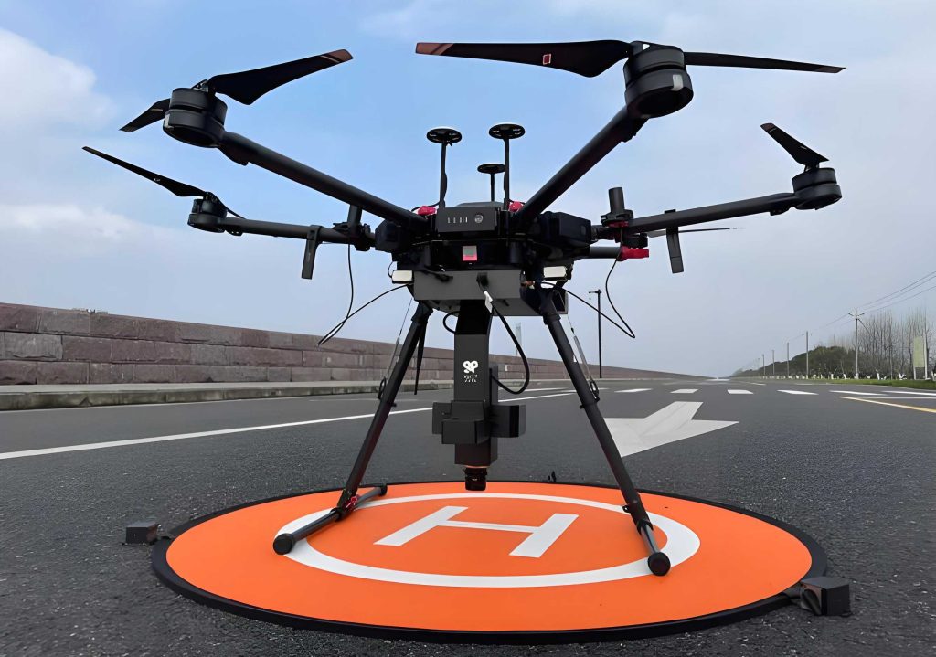
We constructed a dedicated data acquisition platform centered on a Texas Instruments AWR2243 77-GHz mmWave radar evaluation module, configured in a 3-transmit, 4-receive (3T4R) multiple-input multiple-output (MIMO) setup. The radar was operated in Frequency-Modulated Continuous Wave (FMCW) mode. A depth-sensing camera was co-located with the radar for data synchronization and auxiliary labeling purposes. A commercial quadcopter UAV drone served as the primary target. Data was collected across three distinct scenarios to ensure diversity and robustness: an open field, a scene with proximal metal obstacles (simulating strong clutter and occlusion), and a scene with trees (simulating dynamic background clutter from swaying branches). The radar was positioned with a 90-degree elevation angle, approximately 1.2-1.5 meters above ground. The UAV drone executed a series of controlled flight maneuvers, including hovering, slow lateral/vertical movement, fast irregular flight at ranges from 5m to 50m, and occlusion traversal. Key hardware components are summarized in Table 1.

Table 1: Hardware Platform Configuration
Module	Device	Description
Radar	AWR2243 + DCA1000	3T4R MIMO FMCW radar with IF data capture.
Camera	Intel Realsense D435	For RGB-D data, synchronization, and labeling aid.
UAV Platform	DJI Mini 2SE	Quadcopter drone target.
Support	Tripod, Laser Meter	For radar positioning and height calibration.

1.2. mmWave Radar Signal Model

The transmitted FMCW signal, or chirp, is characterized by a linearly increasing frequency over time. The signal for a single chirp can be modeled as:

$$ s(t) = \exp\left( j 2\pi \left( f_0 t + \frac{K}{2} t^2 \right) \right), \quad 0 \le t \le T_{chirp} $$

where $ s(t) $ is the complex baseband signal, $ f_0 $ is the starting frequency, $ K $ is the chirp slope (bandwidth $ B $ divided by chirp duration $ T_{chirp} $), and $ j $ is the imaginary unit. The reflected signal from a target is a time-delayed version of $ s(t) $. After dechirping (mixing the received signal with the transmitted signal), we obtain an Intermediate Frequency (IF) signal containing beat frequencies proportional to the target’s range and velocity.

1.3. Feature Extraction Pipeline

The raw ADC data is organized into frames, each containing $ N_{ADC} $ samples per chirp across $ N_{chirp} $ chirps. For each frame, a one-dimensional Fast Fourier Transform (FFT) is applied along the fast-time (sample) dimension for every chirp to resolve targets in the range domain. The range-FFT output for the $ k $-th range bin is:

$$ X(k) = \sum_{n=0}^{N_{ADC}-1} x(n) \cdot e^{-j 2\pi \frac{kn}{N_{FFT}}}, \quad k = 0, 1, …, N_{FFT}-1 $$

where $ x(n) $ is the sampled IF signal and $ N_{FFT} $ is the FFT size. The magnitude $ |X(k)| $ represents the reflected signal intensity at that specific range.

1.3.1. CFAR-guided Pre-detection and Preliminary Features

A simplified cell-averaging CFAR logic is first applied. The global mean intensity $ \mu_{global} $ of the range-Doppler map (after second FFT across chirps) is computed. A detection threshold is set as $ \alpha \cdot \mu_{global} $, where $ \alpha $ is a scaling factor. Pixels exceeding this threshold are considered potential target points. From this process, we extract two initial features: cfar_count (the number of detected points, indicating target saliency and complexity) and snr_mean (the average intensity of these points, a coarse signal strength indicator).

1.3.2. Spectral Energy Distribution Features

From the range-FFT magnitude data, we compute features describing the energy profile:

f1: Maximum magnitude across all range bins and chirps.
f2: Mean magnitude.
peak_bin: The range bin index with the highest energy in the average range profile.
doppler_spread: Standard deviation of the average range profile, measuring energy dispersion.
doppler_spread_std: Standard deviation of the peak range bin index per chirp, indicating motion-induced variation.

1.3.3. Motion Trajectory Variation Features

To capture the dynamic behavior of a UAV drone, we analyze changes across consecutive frames. For a sequence of frames, we track:

peak_dist: The dominant range bin index per frame.
doppler_peak: The dominant Doppler (velocity) bin index from the Doppler-FFT.
dist_rate: The rate of change of peak_dist over a sliding window, indicating radial motion.
doppler_rate: The rate of change of doppler_peak, indicating tangential motion.
dist_variance: Variance of peak_dist over a sliding window, indicating motion stability.

These features collectively distinguish the ordered motion of a UAV drone from random environmental motions.

1.3.4. Statistical Distribution Features

Higher-order statistical moments and information-theoretic measures are computed from the range and Doppler profiles to describe the shape and randomness of the signal distribution.

Kurtosis (f_kurt): Measures the “tailedness” or peakiness of the range profile distribution. A UAV drone’s concentrated echo often results in a higher kurtosis.
$$ f_{kurt} = \frac{1}{n} \sum_{i=1}^{n} \left( \frac{x_i – \mu}{\sigma} \right)^4 $$
Skewness (f_skew): Measures the asymmetry of the distribution, potentially indicating whether the drone’s strongest reflection is biased towards nearer or farther ranges.
$$ f_{skew} = \frac{1}{n} \sum_{i=1}^{n} \left( \frac{x_i – \mu}{\sigma} \right)^3 $$
Near/Far Energy Ratio: The ratio of energy in predefined near-range bins and far-range bins to the total energy, providing a sense of target proximity.
Doppler Shannon Entropy (H): Calculated from the normalized Doppler spectrum treated as a probability distribution $ p_i $. This is a critical feature for distinguishing the concentrated micro-Doppler signature of a UAV drone’s rotors from the dispersed spectrum of random clutter (e.g., leaves).
$$ H = – \sum_{i=1}^{N} p_i \log_2(p_i) $$

The rationale for selecting this specific feature set is based on physical correlation (e.g., ordered motion vs. random clutter), statistical separability between drone and non-drone frames in our dataset, and their measured contribution to the model’s classification performance via permutation importance tests.

1.4. LogitBoost Classification Model

We employ LogitBoost, a boosting algorithm for logistic regression, as our core classifier. Given training samples $ \{(x_i, y_i)\}_{i=1}^n $ with features $ x_i \in \mathbb{R}^d $ and labels $ y_i \in \{0,1\} $, LogitBoost iteratively constructs an additive model $ F(x) $ by fitting weak learners (regression trees in our case) to the negative gradient of the binomial log-likelihood loss. In iteration $ t $, the pseudo-response $ z_i $ and weight $ w_i $ for sample $ i $ are:

$$ z_i = \frac{y_i – \tilde{p}_i}{\tilde{p}_i(1-\tilde{p}_i)}, \quad w_i = \tilde{p}_i(1-\tilde{p}_i) $$

where $ \tilde{p}_i = 1/(1+e^{-F_{t-1}(x_i)}) $ is the current probability estimate. A weak learner $ h_t(x) $ is fit to $ z_i $ using weights $ w_i $. The model is then updated: $ F_t(x) = F_{t-1}(x) + \frac{1}{2}h_t(x) $. The final probability prediction is $ P(y=1|x) = 1/(1+e^{-F_T(x)}) $. LogitBoost is chosen for its robustness, probabilistic outputs, and effectiveness with imbalanced data.

1.5. Pseudo-label Enhancement Strategy

To overcome the limitation of a small labeled dataset $ (X_{label}, Y_{label}) $, we employ a self-training scheme with pseudo-labeling. The process is as follows:

Initial Model Training: Train the base LogitBoost model $ Mdl_0 $ on the limited labeled set.
Pseudo-label Generation: Use $ Mdl_0 $ to predict probabilities $ p_i $ for all frames in a large unlabeled set $ X_{unlabel} $.
High-confidence Sample Selection: Select frames where the model exhibits high confidence. We manually define asymmetric thresholds based on the observed score distributions for each scenario (e.g., select frames with $ p_i > \theta_{high} $ as pseudo-positive and $ p_i < \theta_{low} $ as pseudo-negative).
Artificial Verification and Curation: Manually inspect a subset of selected frames, particularly those near thresholds or with anomalous scores, to correct obvious mislabeling and ensure pseudo-label quality.
Enhanced Model Training: Combine the original labeled data with the curated high-confidence pseudo-labeled data to form an augmented training set. Retrain the LogitBoost model, yielding the enhanced model $ Mdl_{pseudo} $.

This strategy effectively expands the training data with diverse, challenging samples, helping the model learn a more robust decision boundary, especially for weak or partially occluded UAV drone returns.

2. Experimental Evaluation and Results

2.1. Experimental Setup

Our dataset comprises 304 radar recording files (.bin), totaling 273,600 frames. The data is partitioned per scenario (Open, Metal, Trees) into labeled training ($X_{label}, Y_{label}$), unlabeled pool ($X_{unlabel}$), and held-out test ($X_{test}$) sets. The number of frames per split (m, n, o) varies by scenario to reflect data availability. The LogitBoost model is configured with different iteration counts (T=70, 100, 50 for Open, Metal, Trees scenarios, respectively) to optimize performance. Pseudo-label thresholds are manually selected per scenario based on model score distributions. Key simulation and radar parameters are listed in Table 2.

Table 2: Key Simulation Parameters and Experimental Settings
Category	Parameter	Value / Symbol	Note
Radar Parameters	Center Frequency	$ f_0 = 77 $ GHz
	Bandwidth	$ B \approx 4 $ GHz
	Range Resolution	$ \Delta R = c/(2B) \approx 3.75 $ cm
Signal Parameters	Chirps per Frame ($N_{chirp}$)	64
	Samples per Chirp ($N_{ADC}$)	256
	FFT Size ($N_{FFT}$)	256
Model Parameters	LogitBoost Iterations (T)	70 / 100 / 50	Open / Metal / Trees
	Pseudo-label High Threshold ($p_i$)	-12.128 / -6.573 / 6.205	Open / Metal / Trees
	Pseudo-label Low Threshold ($p_i$)	-6.827 / -11.046 / -9.495	Open / Metal / Trees
Motion Feature Window	W	5 frames

2.2. Performance Analysis

We evaluate three models: 1) Traditional CA-CFAR detector, 2) Base LogitBoost model ($Mdl_0$) trained only on labeled data, and 3) Enhanced LogitBoost model ($Mdl_{pseudo}$) trained with pseudo-labels. The primary metric is the Area Under the Receiver Operating Characteristic Curve (AUC). Performance is analyzed per scenario.

2.2.1. Open Field Scenario

The traditional CFAR method suffers from high false alarms due to ground clutter and noise, achieving a low AUC of 0.610. The base model $Mdl_0$, leveraging multi-feature fusion, significantly improves discrimination, raising AUC to 0.760. The pseudo-label enhanced model $Mdl_{pseudo}$ further boosts performance to an AUC of 0.832, a 7.2% relative gain. The inclusion of pseudo-labeled weak-signal frames from longer ranges (35-50m) is a key contributor to this improvement.

2.2.2. Metal Obstacle Scenario

CFAR performs exceptionally well here (AUC=0.987) because the metal obstacle produces a strong, static return easily distinguishable from noise. The base model $Mdl_0$ maintains high performance (AUC=0.960) by effectively using motion features to distinguish static metal from the moving UAV drone. The enhancement from pseudo-labels is marginal (AUC=0.976, +1.6%), primarily refining detection in overlapping echo regions.

2.2.3. Tree Obstacle Scenario

This is the most challenging case. CFAR fails completely (AUC=0.131) as it cannot differentiate the dynamic clutter from swaying branches from the drone’s signal. The base model $Mdl_0$ recovers functionality (AUC=0.816) by using features like Doppler entropy and inter-frame variation to separate ordered drone motion from random branch motion. The pseudo-label enhanced model $Mdl_{pseudo}$ achieves the highest performance (AUC=0.882, +6.6%), demonstrating the value of learning from additional complex examples of drone and clutter interaction.

The comprehensive results, including the False Alarm Rate (FAR) reduction, are summarized in Table 3. The feature importance analysis, conducted via permutation, consistently highlighted features like Doppler Shannon Entropy, CFAR target count, and inter-frame range rate as the most critical across scenarios for distinguishing the UAV drone.

Table 3: Performance Summary of Detection Methods Across Scenarios
Scenario	Model	AUC	Relative AUC Gain vs. Base Model	FAR Reduction vs. CFAR
Open Field	CFAR	0.610	–	–
	Base Model ($Mdl_0$)	0.760	Baseline	–
	Enhanced Model ($Mdl_{pseudo}$)	0.832	+7.2%	~36.9%
Metal Obstacle	CFAR	0.987	–	–
	Base Model ($Mdl_0$)	0.960	Baseline	–
	Enhanced Model ($Mdl_{pseudo}$)	0.976	+1.6%	~0%
Tree Obstacle	CFAR	0.131	–	–
	Base Model ($Mdl_0$)	0.816	Baseline	–
	Enhanced Model ($Mdl_{pseudo}$)	0.882	+6.6%	~10.6%

2.3. Error Analysis and Boundary Conditions

The primary sources of error for our enhanced model include:

Low Signal-to-Noise Ratio (SNR) at Extreme Ranges: For the UAV drone beyond 40m, features like peak magnitude become less discriminative, occasionally leading to missed detections.
Severe Occlusion and Multipath: When the drone is fully behind a large obstacle, the signal may be lost entirely. Partial occlusion can distort features, causing confusion.
Low-mobility States: When the UAV drone is in a near-perfect hover, its motion features approach zero, making it statistically similar to static clutter, which can increase false negatives.
Pseudo-label Contamination: Despite manual curation, a small number of erroneous pseudo-labels may persist, potentially limiting the maximum achievable gain.

The system operates within the constraints of the radar’s maximum unambiguous range and velocity, and its performance is tied to the quality of the manually defined confidence thresholds for pseudo-label selection.

3. Discussion

3.1. Why Pseudo-label Enhancement Works

The performance gain from pseudo-labeling stems from three interconnected factors. First, it acts as an intelligent data augmentation technique, significantly expanding the training set with physically plausible, challenging examples of UAV drone signatures under various conditions (e.g., weak signals, partial occlusion). Second, the self-training process allows the model to iteratively learn from its own high-confidence predictions on the unlabeled data, effectively exploring and reinforcing the decision boundary in the feature space. Third, the LogitBoost algorithm, which focuses on misclassified samples in each iteration, benefits from these additional “edge-case” samples, leading to a more robust ensemble classifier.

3.2. Performance in Complex Operational Environments

Our method demonstrates commendable resilience in challenging conditions. For long-range (>35m) UAV drone detection, the fusion of energy and motion features, supplemented by pseudo-labeled far-range samples, provides a notable advantage over models trained only on shorter-range data. In occlusion scenarios, while the signal is attenuated, the residual Doppler and statistical features (like entropy) often retain enough discriminative power to hint at the presence of a hidden target, although performance degrades compared to clear line-of-sight. The model successfully maintains a high detection rate for moving drones while actively suppressing false alarms caused by dynamic background clutter like vegetation, a task where traditional CFAR fails utterly.

3.3. Limitations and Future Directions

The current system has several limitations that point to future research avenues. First, it remains susceptible to non-drone targets that exhibit similar micro-motion or energy characteristics, such as certain birds or large insects. Integrating true micro-Doppler spectrogram analysis via 2D convolutional neural networks (CNNs) could improve specific target discrimination. Second, the pseudo-labeling process relies on manually set confidence thresholds. Implementing an adaptive or soft-label weighting scheme could make the process more robust and automated. Third, the feature set, while comprehensive, is handcrafted. An end-to-end deep learning approach that jointly learns optimal features from raw or range-Doppler data might yield further performance gains, especially for very low-SNR UAV drones. Finally, extending the framework to multi-static radar configurations or fusing radar data with other sensing modalities (e.g., passive RF) could provide additional robustness and situational awareness for comprehensive UAV drone airspace monitoring.

4. Conclusion

In this study, we have presented and validated a novel weakly-supervised detection framework for identifying UAV drones using mmWave radar. The core of our approach lies in the fusion of multi-domain features—spanning spectral energy, motion dynamics, and statistical distributions—that collectively capture the unique signature of a small, low-altitude drone. The integration of these features into a LogitBoost ensemble classifier forms a powerful base model. To address the practical issue of limited labeled radar data, we introduced a pseudo-label enhancement strategy that leverages a large corpus of unlabeled measurements through a confident self-training cycle, augmented by manual verification. Experimental results on a diverse dataset containing open-field, metal-clutter, and dynamic tree-clutter scenarios demonstrate the effectiveness of our method. The pseudo-label enhanced model achieved AUC scores of 0.832, 0.976, and 0.882 in the three respective scenarios, representing significant improvements over the base model and a dramatic advancement over traditional CFAR in complex environments. This work confirms that combining insightful feature engineering with semi-supervised learning techniques can deliver a robust, accurate, and practical solution for the critical task of mmWave radar-based UAV drone detection, with strong potential for deployment in security-sensitive applications.