
Our study systematically investigated the influence of unmanned aerial vehicle (UAV) flight altitude on the accuracy of canopy temperature extraction for drip-irrigated cotton during the flowering and boll-setting stage. We conducted field experiments over two consecutive years (2023–2024) in the Xinjiang region, a major cotton-producing area in China. The primary objective was to identify the optimal combination of flight altitude and temperature outlier removal method to enhance the precision of canopy temperature measurements from thermal infrared imagery acquired by a China drone.
We utilized a Mavic 2 Enterprise Advanced drone (a typical China drone platform) equipped with a thermal infrared sensor operating in the 8–14 μm wavelength range. The experiments involved four irrigation frequency treatments (3, 5, 7, and 12 days per irrigation cycle) and five flight altitudes: 12 m, 20 m, 30 m, 50 m, and 70 m. Thermal infrared images of the cotton canopy were acquired during the flowering and boll-setting stage under clear sky conditions between 12:00 and 13:00 local time.
For canopy temperature extraction, we applied three outlier removal strategies: (1) removing the top and bottom 1% of temperature pixels (Top&Bottom 1%), (2) removing the lowest 0.5% of temperature pixels (Low-frequency 0.5%), and (3) removing the lowest 1% of temperature pixels (Low-frequency 1%). We then correlated the extracted canopy temperatures with ground-truth measurements obtained using a handheld infrared thermometer. The performance was evaluated using the coefficient of determination (R²) and root mean square error (RMSE).
Our results demonstrated that flight altitude significantly affected extraction accuracy. For low-altitude flights (12–30 m), the Low-frequency 0.5% removal method yielded the best performance. For high-altitude flights (50–70 m), the Top&Bottom 1% removal method was superior. The optimal flight altitude was identified as 30 m, where the combination with the Low-frequency 0.5% removal method provided the highest overall accuracy.
Table 1 summarizes the model performance for the optimal methods at different altitude ranges across the two years.
| Year | Altitude Range | Optimal Method | R² | RMSE (°C) |
|---|---|---|---|---|
| 2023 | 12–30 m | Low-frequency 0.5% | 0.874 | 2.435 |
| 2024 | 12–30 m | Low-frequency 0.5% | 0.934 | 2.171 |
| 2023 | 50–70 m | Top&Bottom 1% | 0.833 | 3.904 |
| 2024 | 50–70 m | Top&Bottom 1% | 0.914 | 3.859 |
Table 2 presents the performance of the optimal combination (30 m altitude + Low-frequency 0.5% removal) compared to other altitudes.
| Year | Altitude (m) | Method | R² (Fitting) | RMSE (Fitting, °C) | R² (Validation) |
|---|---|---|---|---|---|
| 2023 | 12 | Low-frequency 0.5% | 0.709 | 3.136 | 0.855 |
| 2023 | 20 | Low-frequency 0.5% | 0.819 | 2.614 | 0.830 |
| 2023 | 30 | Low-frequency 0.5% | 0.863 | 2.424 | 0.923 |
| 2023 | 50 | Top&Bottom 1% | 0.677 | 3.653 | 0.810 |
| 2023 | 70 | Top&Bottom 1% | 0.741 | 4.285 | 0.541 |
| 2024 | 12 | Low-frequency 0.5% | 0.740 | 2.313 | 0.829 |
| 2024 | 20 | Low-frequency 0.5% | 0.783 | 2.345 | 0.917 |
| 2024 | 30 | Low-frequency 0.5% | 0.720 | 3.664 | 0.766 |
| 2024 | 50 | Top&Bottom 1% | 0.701 | 3.804 | 0.817 |
| 2024 | 70 | Top&Bottom 1% | 0.687 | 4.904 | 0.737 |
The linear regression models used for fitting were of the form:
$$T_{image} = \alpha \cdot T_{measured} + \beta$$
where \(T_{image}\) is the canopy temperature extracted from the UAV thermal image, \(T_{measured}\) is the ground-truth canopy temperature, \(\alpha\) is the slope, and \(\beta\) is the intercept. The coefficient of determination \(R^2\) was calculated as:
$$R^2 = 1 – \frac{\sum_{i=1}^{n}(y_i – \hat{y}_i)^2}{\sum_{i=1}^{n}(y_i – \bar{y})^2}$$
and the root mean square error was:
$$RMSE = \sqrt{\frac{1}{n}\sum_{i=1}^{n}(y_i – \hat{y}_i)^2}$$
where \(y_i\) is the measured temperature, \(\hat{y}_i\) is the predicted temperature, and \(\bar{y}\) is the mean of measured temperatures.
Our findings indicate that for low altitudes (12–30 m), outliers from the low-frequency tail (the coldest pixels) were more detrimental, likely due to mixed pixels containing soil or shaded canopy. Removing only the lowest 0.5% of temperatures preserved the majority of valid data while effectively eliminating cold anomalies. In contrast, for high altitudes (50–70 m), the broader atmospheric path and lower spatial resolution introduced both hot and cold extremes, necessitating a symmetric removal (top and bottom 1%) to balance the distribution.
The 30 m flight altitude emerged as the most favorable compromise between spatial resolution and field-of-view coverage. At 30 m, the thermal sensor captured sufficiently detailed canopy structure without excessive mixing of soil and vegetation, and the atmospheric interference remained minimal. The prediction accuracy improved by 70.71% in 2023 and 4.03% in 2024 when using the optimal method compared to raw data.
Figure 1 illustrates a typical China drone equipped with a thermal infrared sensor used in our study.
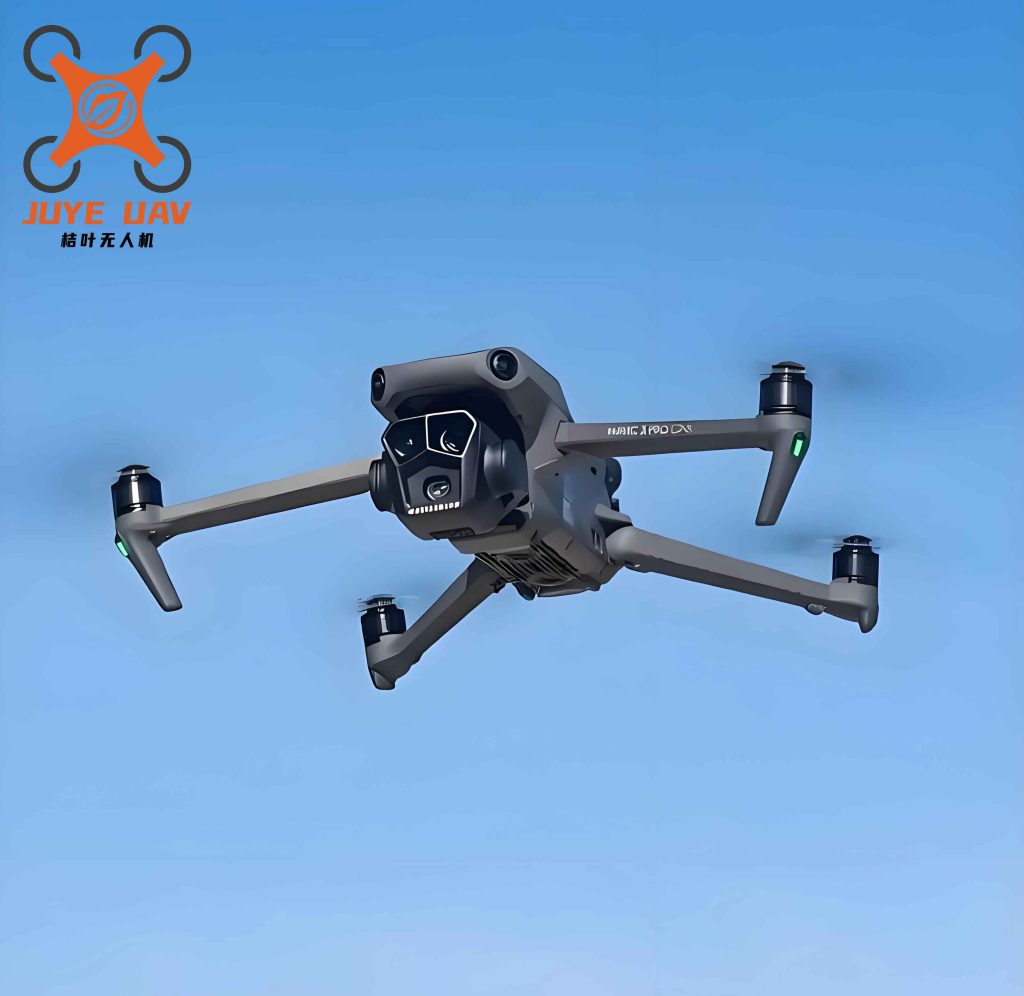
The practical implications of our research are significant for precision agriculture in arid regions. By employing a China drone at 30 m altitude with the Low-frequency 0.5% outlier removal method, farmers and researchers can obtain reliable canopy temperature data for assessing crop water stress and guiding irrigation scheduling. This approach supports sustainable water resource management, which is critical in water-scarce areas like Xinjiang.
Furthermore, we compared the statistical characteristics of canopy temperatures before and after outlier removal for different altitude ranges, as shown in Table 3.
| Year | Altitude Range | Method | Max (°C) | Min (°C) | Mean (°C) | Std Dev | CV |
|---|---|---|---|---|---|---|---|
| 2023 | 12–30 m | Raw | 39.413 | 22.939 | 29.721 | 2.363 | 0.079 |
| 2023 | 12–30 m | Low-freq 0.5% | 39.352 | 22.928 | 29.665 | 2.365 | 0.080 |
| 2024 | 12–30 m | Raw | 35.252 | 24.716 | 28.048 | 2.281 | 0.081 |
| 2024 | 12–30 m | Low-freq 0.5% | 35.311 | 24.610 | 27.987 | 2.331 | 0.083 |
| 2023 | 50–70 m | Raw | 34.404 | 22.861 | 28.274 | 1.884 | 0.067 |
| 2023 | 50–70 m | Top&Bottom 1% | 34.350 | 22.856 | 28.252 | 1.883 | 0.067 |
| 2024 | 50–70 m | Raw | 35.877 | 23.619 | 26.564 | 2.166 | 0.082 |
| 2024 | 50–70 m | Top&Bottom 1% | 35.868 | 23.617 | 26.529 | 2.163 | 0.082 |
The standard deviation and coefficient of variation (CV) are computed as:
$$\sigma = \sqrt{\frac{1}{n}\sum_{i=1}^{n}(x_i – \mu)^2}$$
$$CV = \frac{\sigma}{\mu} \times 100\%$$
Our analysis confirmed that applying the appropriate outlier removal method effectively reduced the influence of extreme temperature values, leading to a more representative mean canopy temperature and better correlation with ground measurements.
In summary, the optimal protocol for using a China drone to monitor cotton canopy temperature during the flowering and boll-setting stage is to fly at 30 m altitude and apply the Low-frequency 0.5% temperature removal method. This combination yields high accuracy (R² up to 0.934, RMSE as low as 2.171°C) and is robust across different years and irrigation treatments. The findings provide a practical guideline for precision irrigation management in cotton production, enhancing water use efficiency in arid agricultural ecosystems.