
The rapid proliferation of fixed-wing and rotary-wing tactical unmanned aerial vehicles (UAVs) has ushered in a new era of aerial threats. Swarm attacks employing small, low-cost drones now represent a primary challenge for modern air defense systems. Recent conflicts have starkly illustrated the devastating potential of drone swarms, capable of overwhelming traditional defenses and executing precision strikes. This evolving threat landscape demands more sophisticated and efficient fire control strategies for anti-aircraft artillery (AAA) systems. Hard-kill methods, particularly using AAA to deploy pre-fragmented munitions that create dense intercepting curtains, remain a crucial and effective means of countering drone swarms. However, the core challenge lies in intelligently allocating limited gun resources to numerous, simultaneous incoming targets to maximize overall defensive effectiveness while conserving assets.
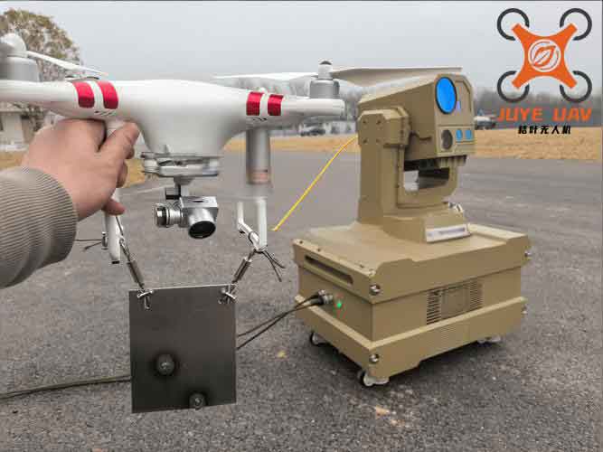
Effective command and control in anti-drone warfare hinges on accurate perception and estimation of the battlefield situation. This involves dynamically assessing the status of both friendly and hostile assets within the operational environment. The ultimate goal is to formulate an optimal engagement strategy. For anti-drone target assignment, this translates to a complex optimization problem. We must process information, evaluate threats, and fuse data to create a coherent tactical picture, enabling rational assignment of each hostile drone to one or more air defense gun units.
Anti-Drone Battlefield Situation Analysis and Modeling
The foundation of effective anti-drone fire assignment is a comprehensive evaluation of the threat. This is a multi-factor decision-making process. Key considerations typically include: the location and value of the assets being defended; and the characteristics of the aerial threat—type, number, altitude, speed, approach direction, and parameters like range and crossing range to the defended asset. Formally, we define a set of drone targets $A = [a_1, a_2, …, a_j]$ and a set of evaluation metrics $U = [u_1, u_2, …, u_m]$. By measuring each target $a_j$ against each metric $u_m$, we construct a decision matrix. From this matrix, we can derive a threat weight vector for the drone targets: $[w_1, w_2, …, w_j]$, where a higher $w_j$ indicates a greater priority for engagement.
A critical tactical constraint in AAA engagements is the fire transition cycle. This refers to the time required for a gun system to engage one target, assess the result, re-orient its barrel, and be ready to engage a subsequent target. The total transition cycle time $t_{zh}$ depends on the firing duration $t_{sj}$ and the re-orientation preparation time $t_{zb}$. The firing duration is relatively fixed and can be expressed as:
$$ t_{sj} = t_{fs} + (n – 1) t_{ls} + t_{pg} $$
where $t_{fs}$ is the time from fire command to muzzle exit, $t_{ls}$ is the cumulative time interval for a burst of $n$ rounds, and $t_{pg}$ is the sum of projectile time-of-flight and kill assessment time. The preparation time $t_{zb}$, including command and physical slew time, is often around 3 seconds. Thus, the complete cycle is:
$$ t_{zh} = t_{fs} + (n – 1) t_{ls} + t_{pg} + t_{zb} $$
This cycle fundamentally limits the rate at which a single gun can engage multiple disparate targets.
Determining the optimal moment to assign a target is crucial. Assigning too early may lead to wasted computation if the target maneuvers; assigning too late reduces the probability of a successful intercept. We define the fire assignment zone as the spatial region where an assigned engagement is feasible, ensuring the projectile and target meet within the gun’s lethal envelope. The far boundary $\rho_{yj}$ and near boundary $\rho_{jj}$ of this zone, considering the target’s approach velocity $v$, altitude $h$, and crossing range $p$, are given by:
$$ \rho_{yj} = \sqrt{ \rho^2_{max} + v^2 (t_{zh} – t_{pg})^2 + 2v(t_{zh} – t_{pg}) \sqrt{\rho^2_{max} – h^2 – p^2} } $$
$$ \rho_{jj} = \sqrt{ \rho^2_{min} + v^2 (t_{zh} – t_{pg})^2 + 2v(t_{zh} – t_{pg}) \sqrt{\rho^2_{min} – h^2 – p^2} } $$
where $\rho_{max}$ and $\rho_{min}$ are the maximum and minimum effective ranges of the gun system. A target must be within this zone for a valid assignment to be made, considering the necessary transition time.
The core metric for evaluating an assignment is the kill probability. For an AAA system, the single-shot kill probability $P$ is typically the product of the hit probability $P_{mz}$ and the conditional probability of kill given a hit $P_{jh}$:
$$ P = P_{mz}P_{jh} $$
While in practice these factors may not be perfectly independent, this assumption simplifies engineering applications. When multiple guns are assigned to a single drone target, and assuming their kill events are independent, the combined kill probability $G(k)$ for $m$ guns with individual kill probabilities $p_i$ is:
$$ G(k) = 1 – \prod_{i=1}^{m} (1 – p_i) $$
This formula is central to evaluating the effectiveness of coordinated anti-drone engagements.
Anti-Drone Target Assignment Model Formulation
Building on these principles, we formulate the anti-drone target assignment optimization model. The primary objective is to maximize the neutralization of threat posed by the drone swarm, prioritizing high-threat and high-probability engagements, while also being mindful of resource expenditure (e.g., ammunition, gun wear). Let us define the following parameters for the model:
- $m$: Number of available anti-aircraft guns.
- $n$: Number of incoming drone targets in the current wave.
- $w_j$: Threat weight of the $j$-th drone target ($j=1,2,…,n$).
- $p_{ij}$: Single-shot kill probability of the $i$-th gun against the $j$-th target.
- $x_{ij}$: Binary decision variable, where $x_{ij}=1$ if gun $i$ is assigned to target $j$, and $0$ otherwise.
The combined kill probability on target $j$ from all assigned guns is therefore:
$$ P_j = 1 – \prod_{i=1}^{m} (1 – p_{ij})^{x_{ij}} $$
The overall assignment effectiveness, aiming to maximize the weighted sum of killed threats, can initially be expressed as:
$$ B(x) = \max \sum_{j=1}^{n} w_j \left[ 1 – \prod_{i=1}^{m} (1 – p_{ij})^{x_{ij}} \right] $$
However, this simple formulation may lead to excessive resource use for marginal gains in kill probability. To balance threat reduction with resource cost, we introduce a satisfaction function $\mu(P_i)$. This function reflects the diminishing utility of assigning excessive firepower to a single target. Its value peaks at a desirable kill probability (e.g., 90%) and decreases if probability becomes excessively high, penalizing over-allocation. Our refined objective function becomes:
$$ B_1(x) = \max \sum_{j=1}^{n} \left\{ w_j \left[ 1 – \prod_{i=1}^{m} (1 – p_{ij})^{x_{ij}} \right] \cdot \mu(P_j) \right\} $$
This function seeks the optimal trade-off between destroying high-threat drones and using guns efficiently in an anti-drone scenario.
The optimization is subject to several practical constraints inherent to anti-drone fire control:
- Gun Capacity Constraint (Targets per Gun): A single gun cannot engage more targets than its fire transition cycle allows within the engagement timeline. If $M_i$ is the maximum number of targets gun $i$ can engage, then:
$$ \sum_{j=1}^{n} x_{ij} \leq M_i, \quad i = 1,2,…,m $$ - Engagement Saturation Constraint (Guns per Target): While multiple guns can be assigned to one drone, there is a practical upper limit $N$ to avoid interference and waste. Also, at least one gun must be assigned to a target to engage it:
$$ 0 < \sum_{i=1}^{m} x_{ij} \leq N \leq m, \quad j = 1,2,…,n $$ - Fire Transition Time Constraint: This is the most complex constraint. If a gun $i$ is assigned to two different targets $j_1$ and $j_2$, the absolute time difference $|\Delta t^{j_1 j_2}_i|$ between their arrivals within the gun’s engagement zone must be greater than or equal to the transition cycle time $t_{zh}$ for the gun to engage both successfully. We model this using an auxiliary parameter $t^{j_1 j_2}_i$ which equals 1 if $|\Delta t^{j_1 j_2}_i| \geq t_{zh}$, and 0 otherwise. The constraint can be formulated as:
$$ \sum_{j_1} \sum_{j_2} x_{ij_1} x_{ij_2} t^{j_1 j_2}_i = \frac{\sum_{j} x_{ij} (\sum_{j} x_{ij} – 1)}{2} $$
This ensures that for every pair of assignments a gun has, the required time separation condition is met. This constraint is critical for realistic modeling of sequential anti-drone engagements.
Algorithm Design: SA-DPSO Hybrid Optimizer
The formulated anti-drone target assignment model is a nonlinear, constrained, combinatorial optimization problem. Traditional methods struggle with such complexity. We employ a hybrid metaheuristic approach combining Discrete Particle Swarm Optimization (DPSO) and Simulated Annealing (SA) to efficiently find high-quality solutions.
DPSO adapts the continuous PSO algorithm to discrete spaces. Each particle’s position $x_{ij}$ is binary, and its velocity represents the probability of $x_{ij}$ being 1. While DPSO is computationally efficient, it can converge prematurely to local optima. SA, on the other hand, has a strong ability to escape local optima by occasionally accepting worse solutions according to a probabilistic criterion controlled by a cooling temperature schedule.
Our proposed SA-DPSO hybrid algorithm integrates these strengths. The DPSO framework provides a directed, population-based search, while the SA mechanism, applied to the particles, allows for localized exploration and helps avoid stagnation. The algorithm proceeds as follows. First, parameters like inertia weight $\omega$, learning factors $c_1, c_2$, swarm size $R$, and SA parameters (initial temperature $T_0$, cooling rate $\lambda$, iterations per temperature $L$) are initialized. The swarm of particles, each representing a candidate assignment matrix $x$, is randomly generated. In the main loop, each particle’s fitness $G_r$ (the value of $B_1(x)$) is evaluated. Personal best ($pbest$) and global best ($gbest$) positions are updated. Then, the SA subroutine is applied to each particle: for $L$ iterations at the current temperature $T$, a neighboring solution $x’_r$ is generated by perturbing the current particle’s position. The change in fitness $\Delta f = G_r – G’_r$ is computed. If $\Delta f < 0$ (improvement), the new solution is accepted. If $\Delta f \geq 0$, it is accepted with probability $\exp(-\Delta f / T)$, allowing controlled uphill moves. This helps refine the solution around the particle’s location. The temperature is then cooled ($T = \lambda T$), and the process repeats until convergence criteria are met. This synergistic combination enhances global search capability and solution quality for the anti-drone assignment problem.
Simulation Analysis and Results
To validate our anti-drone target assignment model and the SA-DPSO algorithm, we conduct a simulation based on a representative scenario. We assume 9 S-70 type UAVs invading in a single wave, defended by 6 AAA units at different locations. Each gun engages with a single burst against a non-maneuvering target. The threat weight $w_j$ for each UAV and the single-shot kill probability $p_{ij}$ for each gun-target pair are given in Table 1.
| Target (j) | Threat ($w_j$) | Kill Probability $p_{ij}$ per Gun (i) | |||||
|---|---|---|---|---|---|---|---|
| Gun 1 | Gun 2 | Gun 3 | Gun 4 | Gun 5 | Gun 6 | ||
| 1 | 0.91 | 0.41 | 0.29 | 0.81 | 0.73 | 0.27 | 0.38 |
| 2 | 0.58 | 0.75 | 0.38 | 0.86 | 0.86 | 0.34 | 0.49 |
| 3 | 0.49 | 0.56 | 0.22 | 0.76 | 0.45 | 0.25 | 0.30 |
| 4 | 0.22 | 0.53 | 0.33 | 0.74 | 0.87 | 0.31 | 0.37 |
| 5 | 0.51 | 0.80 | 0.84 | 0.44 | 0.73 | 0.22 | 0.57 |
| 6 | 0.88 | 0.47 | 0.53 | 0.31 | 0.53 | 0.64 | 0.45 |
| 7 | 0.66 | 0.38 | 0.70 | 0.57 | 0.32 | 0.58 | 0.33 |
| 8 | 0.41 | 0.42 | 0.59 | 0.67 | 0.36 | 0.80 | 0.74 |
| 9 | 0.70 | 0.82 | 0.51 | 0.20 | 0.68 | 0.89 | 0.91 |
The time at which each target enters the engagement zone of each gun (fly-in time, $t_{fl}$ in seconds) is also provided as a matrix. Applying our model with an average transition time $t_{zh}=4$ s and a satisfaction function set to heavily favor kill probabilities above 90%, the SA-DPSO algorithm yields the following optimal assignment matrix $x_{ij}$ (rows: guns i=1..6, columns: targets j=1..9):
$$
x_{ij} =
\begin{bmatrix}
0 & 1 & 1 & 1 & 1 & 0 & 0 & 0 & 0\\
0 & 0 & 0 & 0 & 1 & 1 & 1 & 0 & 0\\
1 & 1 & 1 & 0 & 0 & 0 & 1 & 0 & 0\\
1 & 0 & 1 & 1 & 0 & 1 & 0 & 0 & 0\\
0 & 0 & 0 & 0 & 0 & 1 & 1 & 1 & 0\\
0 & 0 & 0 & 0 & 0 & 0 & 0 & 1 & 1
\end{bmatrix}
$$
This assignment satisfies all fire transition time constraints. The resulting combined kill probability for each target is:
$$ P = [84.87\%, 95.80\%, 94.20\%, 93.99\%, 96.80\%, 96.80\%, 92.05\%, 92.52\%, 94.80\%, 91.00\%] $$
All targets achieve a kill probability near or above the 90% threshold, demonstrating the model’s effectiveness in the anti-drone context.
To benchmark our SA-DPSO algorithm, we compare its performance over 20 simulation runs against the standard DPSO and a classic Genetic Algorithm (GA). The key results are summarized in Table 2. The convergence curves show that SA-DPSO finds a better solution faster and more consistently than the other two methods.
| Metric | SA-DPSO (Avg) | DPSO (Avg) | GA (Avg) | SA-DPSO (Best) |
|---|---|---|---|---|
| Assignment Effectiveness $B(x)$ | 5.031 | 4.958 | 4.833 | 5.031 |
| Avg. Targets Engaged per Gun | 3.3 | 3.6 | 4.1 | 3.3 |
The SA-DPSO algorithm achieves the highest average and best-found assignment effectiveness $B(x)$. Crucially, it does so while requiring the fewest average engagements per gun (3.3). Compared to GA and DPSO, it reduces the average gun workload by approximately 9.1% and 24%, respectively. This means our approach not only delivers superior overall threat reduction but also minimizes the operational burden on each anti-drone artillery unit, allowing for sustained defense. The faster and more stable convergence further confirms SA-DPSO as a robust and efficient solver for this complex anti-drone fire assignment problem.
Conclusion
In this work, we have addressed the critical challenge of optimal target assignment for anti-aircraft artillery against drone swarms. We proposed a comprehensive multi-factor model that incorporates threat assessment, realistic fire transition cycles, engagement zone boundaries, and kill probability calculations. The model’s objective function intelligently balances maximizing threat destruction with minimizing resource expenditure through a satisfaction function. To solve this complex nonlinear optimization problem, we developed a hybrid SA-DPSO algorithm that effectively combines the global search guidance of swarm intelligence with the local escape capability of simulated annealing. Simulation results demonstrate that our model produces practical, constraint-satisfying assignment plans that achieve high kill probabilities across all threats. Furthermore, the SA-DPSO optimizer outperforms standard DPSO and GA in both solution quality and convergence efficiency, while also reducing the average engagement load on individual guns. This research provides a solid, computationally efficient framework for decision-support in anti-drone air defense, offering valuable insights for both system design and operational deployment of gun-based counter-swarm defenses.