
In industrial applications, the use of quadrotor drones as airborne platforms to perform various tasks holds significant potential. The twin propeller propulsion system suspended beneath a quadrotor drone represents a novel working platform that leverages the advantages of quadrotor drones, such as compact size, high maneuverability, and vertical take-off and landing capabilities. By controlling the output of motors on both sides of the propulsion system, the platform can achieve specified spatial positions, enabling it to replace human labor in hazardous environments. However, this system faces challenges due to strong coupling effects and susceptibility to external disturbances, such as sudden thrust forces, which can compromise stability and precision. This research addresses these issues by proposing an optimal control strategy integrated with a disturbance observer to enhance the position response accuracy and anti-interference capability of the propulsion system.
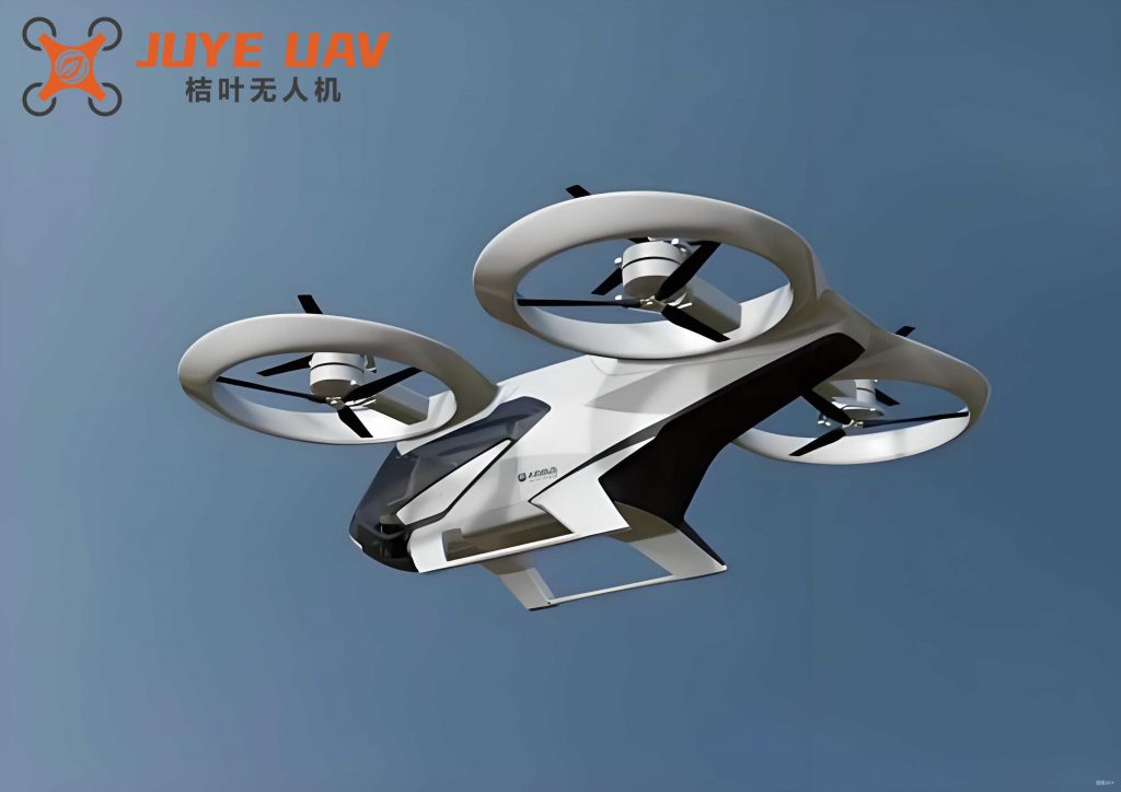
The twin propeller propulsion system under a quadrotor drone operates in a dynamic, suspended environment, requiring real-time adjustment of spatial positions based on control commands from an upper computer. This ensures that the system maintains precise positional output. A key challenge is minimizing the impact of random external disturbances while guaranteeing dynamic tracking performance. To solve this problem, I present a method utilizing an optimal controller with a disturbance observer. The disturbance thrust observer is designed using pole placement to estimate external干扰 thrust in real-time, and feedforward compensation is applied to reduce its effect on the system. An optimal controller is then designed to balance system error and control input, ensuring robust stability of the overall feedback system. Simulation results demonstrate that the optimized system exhibits smaller overshoot and shorter recovery time under disturbances, confirming the effectiveness of the proposed approach in compensating for external perturbations and improving the propulsion system’s performance.
The quadrotor drone’s twin propeller propulsion system is a strongly coupled system. When suspended from the airborne platform, it is prone to sudden干扰 thrusts in the spatial environment, affecting its ability to maintain a stable working posture. Appropriate control strategies are essential for ensuring speed response, fast position tracking, and stable output. Overcoming external thrust disturbances and parameter variations is a critical research direction. Existing methods, such as PID control, sliding mode control, robust control, and neural network control, have been employed in engineering applications. However, for simplified models, these strategies may not achieve the desired control performance. Therefore, this study builds upon existing control strategies by designing an optimal control system based on a突变 thrust observer, using an LQR controller for the outer loop to suppress observer errors and enhance tracking accuracy.
The twin propeller propulsion system requires that during quadrotor drone flight, by controlling the differential thrust outputs of the two side motors, pitching and yawing motions are achieved to ensure the platform reaches desired spatial work positions. The system exhibits strong coupling in both pitching and yawing directions. Through state feedback decoupling analysis, the system can be separately controlled in these directions. Here, I focus on the pitching direction as an example to illustrate the control system design process. The overall control structure is depicted in Figure 1, but for brevity, the details are described in the text.
When the thrusts generated by the motors on both sides of the propulsion system are equal, the force analysis simplifies to a pendulum-like model. Let point O be the suspension point at a distance \( l \) from the system’s center, \( \theta \) be the angle from the vertical direction at equilibrium, \( m \) be the total mass, \( F \) be the combined thrust from both motors, and \( I_o \) be the moment of inertia about point O. Neglecting air resistance and other minor frictional forces, and assuming rigid body components, the system’s motion equation is derived using Newton’s law:
$$ F \cdot l – m g l \cdot \sin \theta = I_o \cdot \ddot{\theta} $$
Rewriting this equation:
$$ \ddot{\theta} + \frac{m g l \cdot \sin \theta}{I_o} = \frac{F \cdot l}{I_o} $$
This equation is nonlinear. For linearization, assuming small oscillations where \( \sin \theta \approx \theta \), the equation simplifies to:
$$ \ddot{\theta} + \frac{m g l \cdot \theta}{I_o} = \frac{F \cdot l}{I_o} $$
Applying Laplace transform, the transfer function for the pitching direction is:
$$ \frac{\theta(s)}{F(s)} = \frac{\frac{l}{I_o}}{s^2 + \frac{m g l}{I_o}} $$
where \( F = F_1 + F_2 \), with \( F_1 \) and \( F_2 \) being the thrusts from the two motors. Based on measurements, the system parameters are: \( I_o = 0.36 \, \text{kg} \cdot \text{m}^2 \), \( l = 0.6 \, \text{m} \), and \( m = 1 \, \text{kg} \). These parameters are summarized in Table 1.
| Parameter | Symbol | Value | Unit |
|---|---|---|---|
| Moment of Inertia | \( I_o \) | 0.36 | kg·m² |
| Distance to Center | \( l \) | 0.6 | m |
| Total Mass | \( m \) | 1 | kg |
| Gravitational Acceleration | \( g \) | 9.81 | m/s² |
Designing a control system involves implementing strategies to achieve required speed response and position tracking. In this design, to counteract external突变 thrust disturbances, a disturbance thrust observer is designed to estimate and compensate for perturbations via feedforward, enabling rapid disturbance rejection and improved response accuracy for the quadrotor drone platform.
Typically, quadrotor drones are powered by lithium batteries, and the system’s operational duration is closely tied to energy consumption rates. By designing an optimal LQR controller, a balance between energy expenditure and positional output is achieved, making the system more efficient and stable. Optimal control is a vital component of modern control theory, focusing on selecting admissible controls that guide the system according to technical requirements while optimizing a given performance index. For the actual control system, the reference input is the desired angle \( \theta_0 \). The error \( e(t) = \theta_0 – \theta(t) \) necessitates a position loop controller \( K(s) \) to ensure干扰 rejection, measurement noise suppression, and robust stability of the closed-loop system.
Consider the system represented in state-space form:
$$ \dot{x} = A x + B u $$
$$ z = H_1 x $$
The goal is to find a control law \( u = -K x \) that minimizes the performance index:
$$ \Gamma = \int_0^\infty \left[ \rho z^2(t) + u^2(t) \right] dt $$
where \( z \) is the output tracking error, and \( \rho \) is a weighting coefficient. By selecting matrix \( H_1 \), the optimal closed-loop poles are chosen to keep tracking error small, and \( \rho \) is tuned to balance tracking error and control effort. In this design, the output \( z \) is taken as \( 2\theta + \dot{\theta} \), which penalizes both position and velocity. Setting \( Q = \rho H_1^T H_1 \) and \( R = 1 \), and after iterative tuning, \( \rho = 12 \) is selected. Using MATLAB’s `lqr()` function, the optimal control gain is obtained:
$$ K = \begin{bmatrix} 2.1306 & 3.7844 \end{bmatrix} $$
Thus, the loop transfer function for the controller is:
$$ K(sI – A)^{-1}B = \frac{6.32s + 3.56}{s^2 + 16.35} $$
The controller parameters are summarized in Table 2.
| Parameter | Symbol | Value |
|---|---|---|
| Weighting Coefficient | \( \rho \) | 12 |
| Control Gain | \( K \) | [2.1306, 3.7844] |
| Loop Transfer Function | \( K(sI-A)^{-1}B \) | \( \frac{6.32s + 3.56}{s^2 + 16.35} \) |
To ensure stable output in the pitching motion, an optimal controller is used for regulation. Integrating a suitably designed load observer into the control system can effectively mitigate the impact of load variations on control quality. When the horizontal thrusts from both motors are equal, the system tilts in the XOZ plane. Assuming a sudden disturbance load \( F_l \) opposite to the motor thrust direction, the system’s equation becomes:
$$ F \cdot l – m g l \cdot \sin \theta – F_l = I_o \cdot \ddot{\theta} $$
Linearizing using the small-angle approximation:
$$ I_o \cdot \ddot{\theta} + m g l \cdot \theta + F_l = F \cdot l $$
For the reduced-order observer design, the system’s state variables are chosen as the pitch angle \( \theta \), angular velocity \( \dot{\theta} \), and disturbance thrust \( F_l \). The motor thrust \( F \) is the input, and the pitch angle \( \theta \) is the output. The third-order state equation is:
$$ \begin{bmatrix} \dot{\theta} \\ \ddot{\theta} \\ \dot{F}_l \end{bmatrix} = \begin{bmatrix} 0 & 1 & 0 \\ -\frac{m g}{I_o} & 0 & -\frac{1}{I_o} \\ 0 & 0 & 0 \end{bmatrix} \begin{bmatrix} \theta \\ \dot{\theta} \\ F_l \end{bmatrix} + \begin{bmatrix} 0 \\ \frac{l}{I_o} \\ 0 \end{bmatrix} F $$
Output: \( y = \theta \). Partition the state vector into measurable part \( x_1 = \theta \) and to-be-estimated part \( x_2 = [\dot{\theta}, F_l]^T \). Then:
$$ \begin{aligned} \dot{x}_1 &= A_{11} x_1 + A_{12} x_2 + B_1 u \\ \dot{x}_2 &= A_{21} x_1 + A_{22} x_2 + B_2 u \\ y &= x_1 \end{aligned} $$
with \( A_{11} = 0 \), \( A_{12} = [1, 0] \), \( A_{21} = [-\frac{m g}{I_o}, 0]^T \), \( A_{22} = \begin{bmatrix} 0 & -\frac{1}{I_o} \\ 0 & 0 \end{bmatrix} \), \( B_1 = 0 \), and \( B_2 = [\frac{l}{I_o}, 0]^T \). Following reduced-order observer design methods, the observer is given by:
$$ \dot{x}_3 = (A_{22} – L A_{12}) \hat{x}_2 + (A_{21} – L A_{11}) y + (B_2 – L B_1) u $$
where \( x_3 \triangleq \hat{x}_2 – L y \) is introduced to avoid differentiation that could amplify noise. The observer equation becomes:
$$ \dot{x}_3 = N_1 \hat{x}_2 + N_2 y + N_3 u $$
with \( N_1 = A_{22} – L A_{12} = \begin{bmatrix} -l_1 & -\frac{1}{I_o} \\ -l_2 & 0 \end{bmatrix} \), \( N_2 = A_{21} – L A_{11} = [-\frac{m g}{I_o}, 0]^T \), and \( N_3 = B_2 – L B_1 = [\frac{l}{I_o}, 0]^T \). The estimate \( \hat{x}_2 \) is recovered as:
$$ \hat{x}_2 = x_3 + L y = \begin{bmatrix} I & L \end{bmatrix} \begin{bmatrix} x_3 \\ y \end{bmatrix} $$
The observer structure is shown in Figure 3. Substituting the matrices, the observer model equations are:
$$ \begin{aligned} \dot{\hat{\theta}} – l_1 \dot{y} &= -l_1 \hat{\dot{\theta}} – \frac{\hat{F}_l}{I_o} – \frac{m g}{I_o} y – \frac{l}{I_o} u \\ \dot{\hat{F}}_l – l_2 \dot{y} &= -l_2 \hat{\dot{\theta}} \end{aligned} $$
Simplifying:
$$ \begin{aligned} \dot{\hat{\theta}} – l_1 \dot{y} &= -l_1 \hat{\dot{\theta}} – A_1 \hat{F}_l – A_2 y – A_3 u \\ \dot{\hat{F}}_l – l_2 \dot{y} &= -l_2 \hat{\dot{\theta}} \end{aligned} $$
where \( A_1 = \frac{1}{I_o} \), \( A_2 = \frac{m g}{I_o} \), and \( A_3 = \frac{l}{I_o} \).
The feedback gain \( L = [l_1, l_2]^T \) is chosen to place the eigenvalues of \( A_{22} – L A_{12} \) at desired locations, ensuring fast estimation convergence without excessive noise sensitivity. The characteristic polynomial of the observer is:
$$ \alpha(s) = \det(sI – (A_{22} – L A_{12})) = s^2 + l_1 s – \frac{l_2}{I_o} $$
If desired eigenvalues are \( \lambda_1 \) and \( \lambda_2 \), then:
$$ \alpha(s) = (s – \lambda_1)(s – \lambda_2) = s^2 – (\lambda_1 + \lambda_2)s + \lambda_1 \lambda_2 $$
Comparing coefficients:
$$ l_1 = -(\lambda_1 + \lambda_2), \quad l_2 = -(\lambda_1 \lambda_2) I_o $$
As a rule of thumb, observer poles are set 2 to 6 times faster than controller poles to ensure rapid error decay without introducing excessive sensor noise. In this design, observer poles are set at twice the speed of the controller poles. The controller poles are derived from the LQR design, leading to observer poles:
$$ \lambda_1 = -6.4 + 6.3j, \quad \lambda_2 = -6.4 – 6.3j $$
Substituting into the equations yields \( L \). The observer parameters are summarized in Table 3.
| Parameter | Symbol | Value |
|---|---|---|
| Observer Poles | \( \lambda_1, \lambda_2 \) | -6.4 ± 6.3j |
| Feedback Gain | \( l_1 \) | 12.8 |
| Feedback Gain | \( l_2 \) | 81.0 |
| Observer Matrices | \( N_1, N_2, N_3 \) | As derived above |
Through the designed controller and observer, a simulation model is built in Simulink to verify system performance. The observer’s tracking特性 and disturbance rejection capabilities are tested. In the simulation, a disturbance thrust of 5 N is applied at 0.3 s and removed after 2 s, and a desired pitch angle of 10° is set. The estimated disturbance thrust from the reduced-order observer is shown in Figure 5. The results indicate that the estimated thrust closely matches the applied disturbance, confirming the observer’s accuracy.
By feeding forward the estimated disturbance thrust for compensation, the system response is shown in Figure 6. To clearly compare the disturbance rejection with and without the observer, the response during the disturbance period is magnified. The results show that after setting the target angle, the settling time is 1.2 s with no overshoot. Without the observer, the disturbance causes a pitch fluctuation of 0.5° with a settling time of 1.8 s. With the observer, the fluctuation reduces to 0.1° and the settling time to 0.3 s. Clearly, incorporating disturbance thrust observation and feedforward compensation reduces position波动 and adjustment time, enhancing the anti-disturbance capability of the twin propeller propulsion system for quadrotor drones.
The simulation outcomes underscore the efficacy of the proposed control strategy. The integration of an optimal LQR controller with a reduced-order disturbance observer significantly improves the robustness and precision of the quadrotor drone’s propulsion system. This approach is particularly beneficial for applications requiring high stability under dynamic conditions, such as aerial manipulation or inspection tasks. Future work could explore adaptive tuning of the observer gains or extension to multi-axis control for full spatial maneuvering. Additionally, real-world testing on a physical quadrotor drone platform would validate the simulation findings and further refine the control algorithms.
In conclusion, for the twin propeller propulsion control system under a quadrotor drone, this study successfully designed an anti-disturbance optimal controller by feedforward compensating the disturbance thrust estimated by a reduced-order observer. The key findings are: (1) The reduced-order disturbance thrust observer, utilizing directly measurable angle variables as known states, is feasible and provides accurate estimates of干扰 thrust. (2) Incorporating the observer’s estimates via feedforward compensation into the optimal control strategy is effective. (3) The proposed system reduces pitch fluctuations caused by disturbance thrust, shortens adjustment times during sudden disturbances, and strengthens the anti-disturbance capability of the propulsion system. This research contributes to advancing control methodologies for quadrotor drone-based platforms, enabling more reliable and precise operations in challenging environments.
Further analyses could involve sensitivity studies on parameter variations, such as changes in mass or inertia, to evaluate the controller’s robustness. Moreover, comparing the proposed method with other advanced control techniques, like model predictive control or adaptive sliding mode control, would provide insights into relative performance. The implementation of such control systems on actual quadrotor drones requires consideration of computational resources and sensor limitations, which are important practical aspects for deployment.
To summarize the overall system design, Table 4 presents a comprehensive overview of the components and their functions in the context of quadrotor drone applications.
| Component | Function | Key Features |
|---|---|---|
| Twin Propeller System | Provides thrust for position adjustment | Suspended under quadrotor drone, coupled dynamics |
| Optimal LQR Controller | Minimizes tracking error and control effort | Balances energy consumption and precision |
| Reduced-Order Observer | Estimates external disturbance thrust | Uses pole placement for fast, noise-resistant estimation |
| Feedforward Compensation | Cancels estimated disturbances | Enhances anti-interference capability |
| Simulation Framework | Validates control performance | Demonstrates reduced overshoot and settling time |
The mathematical foundation of the control design can be further elaborated through additional equations. For instance, the overall closed-loop system dynamics with observer compensation can be expressed as follows. Let the system state be \( x = [\theta, \dot{\theta}, F_l]^T \), and the control input \( u = F \). With the observer providing estimate \( \hat{F}_l \), the compensated control law becomes:
$$ u = -K \begin{bmatrix} \theta \\ \dot{\theta} \end{bmatrix} – \hat{F}_l \cdot \text{feedforward gain} $$
Assuming perfect estimation, the disturbance effect is canceled, leading to improved tracking. The error dynamics of the observer can be analyzed by defining estimation error \( e = x_2 – \hat{x}_2 \), which satisfies:
$$ \dot{e} = (A_{22} – L A_{12}) e $$
Thus, by proper selection of \( L \), the error converges exponentially. This theoretical assurance underpins the practical simulation results.
In terms of implementation on a quadrotor drone, the control algorithm must be computationally efficient to run in real-time on embedded systems. The LQR controller requires only matrix multiplications, and the reduced-order observer involves simple differential equations, both feasible for modern microcontrollers. Moreover, the use of such control strategies can be extended to other drone configurations, such as hexacopters or octorotors, with appropriate model adjustments.
The role of quadrotor drones in industrial applications continues to expand, and advancements in control systems like the one presented here are crucial for unlocking their full potential. By ensuring precise and stable operation under disturbances, these systems can perform complex tasks in construction, agriculture, search and rescue, and environmental monitoring. The integration of optimal control and disturbance observation represents a step forward in making quadrotor drone platforms more autonomous and reliable.
Finally, it is worth noting that the simulation environment allows for extensive testing without physical risks. Parameters can be varied to study edge cases, and the control design can be iteratively refined. For future work, hardware-in-the-loop simulations could bridge the gap between simulation and real-world deployment, further validating the approach for actual quadrotor drone systems.