
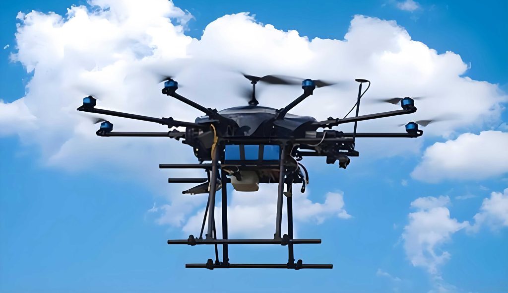
Unmanned aerial vehicles (UAVs), especially quadrotors, have become indispensable tools in modern applications such as precision agriculture, infrastructure inspection, search and rescue, and last-mile delivery. With the rapid development of wireless communication and sensing technologies, the operational scenarios for unmanned aerial vehicles are expanding dramatically. However, this expansion also brings unprecedented challenges: agricultural operations often require flying through densely forested areas, while urban low-altitude missions involve navigating around complex buildings and dealing with electromagnetic interference. In these complex environments, the safety and efficiency of unmanned aerial vehicles heavily depend on the ability to perform real-time obstacle avoidance motion planning. This thesis addresses the obstacle avoidance problem for quadrotor unmanned aerial vehicles in near-ground cluttered environments. I design a complete obstacle avoidance system that integrates a front-end path planner based on a modified A* algorithm and a back-end trajectory optimizer based on an improved minimum-jerk algorithm. The proposed system aims to achieve both fast discrete path search and dynamically feasible, collision-free trajectory generation.
Introduction and Background
The difficulty of obstacle avoidance for unmanned aerial vehicles in complex environments lies in the high density of obstacles and the stringent real-time requirements. Traditional path planning algorithms such as the A* algorithm, though widely used, suffer from high memory consumption and slow search speed when the environment contains a large number of obstacles. Moreover, the path produced by a discrete search algorithm is often piecewise linear and does not satisfy the dynamic constraints of a quadrotor. Therefore, a two-stage approach is commonly adopted: first, a discrete path is searched in the configuration space; second, a trajectory optimization step converts the discrete waypoints into a smooth, time-parametrized trajectory. In this work, I focus on both stages and propose several contributions. First, I present a Jump A* (JA*) algorithm that extends the Jump Point Search (JPS) strategy to three dimensions. This algorithm significantly reduces the number of expanded nodes and shortens the planning time in high-density obstacle maps. Second, I design a pruning algorithm that removes redundant waypoints from the front-end path, allowing for arbitrary directions and reducing the number of turns. Third, I construct safe flight corridors in the UAV flight space to constrain the waypoints. Fourth, I improve the minimum-jerk trajectory generation scheme by replacing the standard fifth-order polynomial with a Bezier curve representation. This modification guarantees that the entire trajectory stays inside a safe convex region, thereby ensuring collision avoidance.
The rest of this article is organized as follows. Section II reviews the fundamentals of path planning and trajectory planning algorithms. Section III describes the JA* algorithm in detail, including the improved heuristic function, the three-dimensional JPS strategy, and the pruning algorithm. Section IV presents the trajectory planning framework, including flight corridor generation and the Bezier-curve-based minimum-jerk optimization. Section V reports simulation results and comparisons. Section VI concludes the work.
Fundamentals of UAV Motion Planning
For unmanned aerial vehicles, motion planning can be formulated as finding a feasible trajectory from an initial state to a goal state while satisfying constraints imposed by the environment and the vehicle dynamics. In this work, the UAV is modeled as a quadrotor with a 12-dimensional state vector
$$ X = [x, y, z, \phi, \theta, \psi, v_x, v_y, v_z, \omega_x, \omega_y, \omega_z]^T, $$
where \(x,y,z\) are the position coordinates, \(\phi,\theta,\psi\) are the Euler angles, \(v_x,v_y,v_z\) are the linear velocities, and \(\omega_x,\omega_y,\omega_z\) are the angular velocities. Using the differential flatness property, the state and control inputs can be expressed in terms of the flat outputs \(x,y,z\) and the yaw angle \(\psi\). This reduces the dimensionality of the planning problem and allows us to plan directly in the output space.
Occupancy Grid Map
The environment is represented as a three-dimensional occupancy grid map. Each voxel is marked as either free or occupied. The resolution of the grid is set to 0.2 m in this work. The UAV is considered as a point after inflating the obstacles by the vehicle radius. The grid map enables efficient collision checking during the path search. In a 3D grid, a node can move to any of its 26 neighbors, as illustrated in the conceptual model. The movement cost depends on the direction: a straight move has cost 1, a diagonal move on a plane has cost \(\sqrt{2}\), and a three-dimensional diagonal move has cost \(\sqrt{3}\).
Classic A* Algorithm
The classic A* algorithm is a heuristic search algorithm that maintains two lists: the open list and the closed list. The cost function for a node \(n\) is
$$ f(n) = g(n) + h(n), $$
where \(g(n)\) is the actual cost from the start node to node \(n\), and \(h(n)\) is the heuristic estimate of the cost from node \(n\) to the goal. Common heuristic functions include the Euclidean distance and the Manhattan distance. However, the Euclidean distance underestimates the true cost on a grid with diagonal moves, leading to more explored nodes. The Manhattan distance overestimates the cost and may yield suboptimal paths. In this work, I adopt a three-dimensional diagonal distance as the heuristic function, which exactly matches the true shortest path cost in a 3D 26-neighbor grid.
Jump Point Search (JPS)
Jump Point Search is an optimization of A* that reduces the number of expanded nodes by exploiting the regularity of the grid. The key idea is to prune redundant neighbors and to generate long jumps in the direction of movement. A node is recognized as a jump point if it has a forced neighbor or if it can reach a jump point in the current direction. The rules for pruning natural neighbors and identifying forced neighbors are based on the relative costs of alternative paths. In this work, I extend the two-dimensional JPS rules to three dimensions, developing a comprehensive set of pruning and jumping strategies for all possible move directions in a 3D grid.
Sampling-Based Methods
For completeness, I also review sampling-based planning algorithms such as RRT (Rapidly-exploring Random Tree) and PRM (Probabilistic Roadmap). These algorithms are probabilistically complete and can handle high-dimensional spaces. However, they tend to produce non-optimal paths and require additional post-processing to improve path quality. In dense obstacle environments, the random sampling strategy often generates many useless samples, leading to high computational cost. Therefore, I choose the deterministic graph-based search as the foundation for the front-end planner.
Trajectory Planning
Trajectory planning aims to generate a smooth, time-parametrized curve that minimizes a certain cost functional while satisfying boundary conditions and dynamic constraints. The minimum-jerk trajectory optimization minimizes the integral of the squared jerk (third derivative of position) over time:
$$ J = \int_{0}^{T} \left\| \frac{d^3 p(t)}{dt^3} \right\|^2 dt. $$
This cost penalizes rapid changes in acceleration, which is beneficial for the stability of gimbaled cameras and the comfort of the flight. The trajectory is often parameterized as a piecewise polynomial. Let the \(i\)-th segment be a fifth-order polynomial
$$ p_i(t) = a_{i,0} + a_{i,1} t + a_{i,2} t^2 + a_{i,3} t^3 + a_{i,4} t^4 + a_{i,5} t^5. $$
Continuity constraints require that the position, velocity, and acceleration be continuous at the segment boundaries. The resulting optimization problem is a quadratic program (QP). However, the optimized polynomial may leave the safe area and collide with obstacles. To avoid this issue, I employ Bezier curves, whose convex hull property guarantees that the entire curve lies within the convex hull of its control points. Therefore, by constraining the control points inside a safe flight corridor, the whole trajectory is guaranteed to be collision-free.
Proposed JA* Path Planning Algorithm
In this section, I present the proposed Jump A* (JA*) algorithm. The algorithm combines a modified heuristic function, a dedicated 3D jump point search strategy, and a pruning post-processing step.
Improved Heuristic Function
The expression for the three-dimensional diagonal distance is derived as follows. Given the current node \(n\) and the goal node \(g\), let
$$ dx = |x_g – x_n|, \quad dy = |y_g – y_n|, \quad dz = |z_g – z_n|. $$
Let \(v_1 \ge v_2 \ge v_3\) be the sorted values of \(dx, dy, dz\). The diagonal distance is
$$ h(n) = \sqrt{3} \cdot v_3 + \sqrt{2} \cdot (v_2 – v_3) + (v_1 – v_2). $$
This heuristic is admissible and consistent, providing a tight lower bound on the true path cost in a 3D 26-neighbor grid. Compared with the Euclidean distance, it better reflects the actual movement cost, thereby reducing the number of expanded nodes without sacrificing optimality.
Three-Dimensional Jump Point Search
In two-dimensional JPS, the movement is classified into straight (horizontal/vertical) and diagonal directions. In three dimensions, we additionally have triagonal movements that change the altitude and both horizontal coordinates simultaneously. The pruning rules depend on the relative position of the parent node and the presence of obstacles. The forced neighbor condition is a node that must be expanded because otherwise an obstacle would block the path. I classify the 3D movement into three categories:
- Straight movement: changing only one coordinate (cost = 1).
- Diagonal movement: changing two coordinates (cost = \(\sqrt{2}\)).
- Triagonal movement: changing three coordinates (cost = \(\sqrt{3}\)).
For each category, the pruning rules are formulated by comparing the cost of reaching a neighbor through the current node versus bypassing it. When no obstacles are present, non-natural neighbors are pruned. When obstacles are present near the current node, some neighbors become forced. The details of the three-dimensional pruning rules are summarized in the following table.
| Movement type | Obstacle case | Forced neighbor condition |
|---|---|---|
| Straight | No obstacle | None |
| Straight | Obstacle beside the current node in the perpendicular plane | The neighbor adjacent to the obstacle in the direction perpendicular to movement |
| Diagonal | No obstacle | None |
| Diagonal | Obstacle adjacent to the current node and the moving direction | The neighbor on the opposite side of the obstacle |
| Triagonal | No obstacle | None |
| Triagonal | Obstacle blocking the intermediate plane | Neighbors that would otherwise be unreachable |
The jump rule is applied recursively. Starting from the current node, the algorithm looks for a jump point along a given direction. A node is a jump point if it has a forced neighbor or if it lies on the goal position. The 3D JPS strategy is implemented by expanding all possible directions (including the vertical dimension) and evaluating the jump points. This approach dramatically reduces the size of the open list compared to classical A*.
Algorithm Workflow
The pseudo-code of the JA* algorithm is presented in Algorithm 1.
| Algorithm 1: JA* Path Planning |
|---|
|
Input: start node \(s\), goal node \(g\), 3D occupancy grid map Output: path from \(s\) to \(g\) 1: Initialize open list with \(s\), set \(g(s)=0\), \(h(s)\) by the 3D diagonal distance. 2: while open list is not empty do 3: pop the node \(n\) with the minimum \(f(n)\) from open list. 4: if \(n\) equals goal \(g\) then 5: reconstruct the path by backtracking and return it. 6: end if 7: expand node \(n\) using the 3D JPS strategy to find a set of jump points \(\{j_1, j_2, \ldots\}\). 8: for each jump point \(j\) do 9: compute tentative \(g(j)\). 10: if \(j\) is not in open list then 11: insert \(j\) into open list. 12: else if tentative \(g(j) < g(j)\) then 13: update \(g(j)\) and the parent of \(j\). 14: end if 15: end for 16: end while 17: return failure. |
Path Pruning Algorithm
The path produced by the JA* algorithm is a sequence of consecutive voxels. Such a path contains many redundant nodes. To reduce the number of waypoints and make the path more suitable for trajectory optimization, I design a pruning algorithm based on line-of-sight collision checking. Starting from the first waypoint, the algorithm checks the straight line to each subsequent waypoint. If the line is collision-free and the line from the first waypoint to the next one collides, the current waypoint is retained. The process repeats from the retained waypoint until the goal is reached. The pseudo-code is given in Algorithm 2.
| Algorithm 2: Path Pruning |
|---|
|
Input: path \(P = [P_1, P_2, \ldots, P_n]\) generated by JA* Output: simplified path \(S\) 1: Initialize \(S = [P_1]\), set \(s = P_1\). 2: for \(i = 2\) to \(n-1\) do 3: if line(s, \(P_i\)) is collision-free and line(s, \(P_{i+1}\)) collides then 4: append \(P_i\) to \(S\). 5: set \(s = P_i\). 6: end if 7: end for 8: append the goal \(P_n\) to \(S\). 9: return \(S\). |
The pruning algorithm effectively removes redundant turn points and shortens the path. In a typical 5 m × 5 m × 5 m map with an obstacle ratio of 0.4, the pruning step reduces the number of waypoints from 8.7 on average to 4.3, while the path length is shortened from 4.498 m to 4.403 m. The additional computation time is only about 0.07 ms, which is negligible.
Improved Minimum-Jerk Trajectory Planning
The front-end path is a polyline consisting of the simplified waypoints. To make the trajectory feasible for the quadrotor, I generate a smooth trajectory using a modified minimum-jerk optimization algorithm. The key issue is that the standard polynomial trajectory may violate the safety constraints. Therefore, I first construct safe flight corridors around the waypoints, then represent the trajectory as a set of Bezier curves whose control points are constrained inside the corridors.
Obstacle Inflation
Before constructing the corridors, I inflate all obstacles by a safety margin equal to the UAV’s radius (approximately 0.2 m). This ensures that the generated trajectory maintains a safe distance from the original obstacles. The inflation operation is applied in all three dimensions.
Safe Flight Corridor Generation
The flight corridor is a series of convex polytopes that contain the simplified path segments. For each segment between two consecutive waypoints \(P_i\) and \(P_{i+1}\), I generate an ellipsoid that has the segment as its principal axis. The ellipsoid is iteratively expanded until it touches an obstacle. At the contact point, a separating plane is constructed. Repeating this process yields a set of half-spaces that form a convex polyhedron. The union of these polyhedra constitutes the safe flight corridor. The ellipsoid is defined as
$$ (p – c)^T E (p – c) \le 1, $$
where \(c\) is the center of the ellipsoid and \(E\) is a symmetric positive definite matrix. The separating planes produce a convex polytope in the form
$$ \{ p \mid A_i p \le b_i, \quad i = 1, \ldots, m \}. $$
Bezier Curve Representation
To guarantee that the optimized trajectory never leaves the safe corridor, I use Bezier curves instead of ordinary polynomials. A Bezier curve of degree \(n\) is defined by \(n+1\) control points \(c_0, c_1, \ldots, c_n\):
$$ B(t) = \sum_{i=0}^{n} C_n^i (1-t)^{n-i} t^i c_i, \quad t \in [0,1]. $$
The convex hull property states that \(B(t)\) lies entirely inside the convex hull of the control points. When multiple Bezier segments are connected to form a trajectory, the continuity of position, velocity, and acceleration can be imposed on the control points. I adopt a quintic Bezier curve (degree 5) for each segment, matching the minimum-jerk requirement.
The transformation matrix from the standard polynomial coefficients to the Bezier control points is given by the following matrix \(\mathbf{M}\) for degree 5:
$$
\mathbf{M} = \begin{bmatrix}
1 & 0 & 0 & 0 & 0 & 0 \\
-5 & 5 & 0 & 0 & 0 & 0 \\
10 & -20 & 10 & 0 & 0 & 0 \\
-10 & 30 & -30 & 10 & 0 & 0 \\
5 & -20 & 30 & -20 & 5 & 0 \\
-1 & 5 & -10 & 10 & -5 & 1
\end{bmatrix}.
$$
For a trajectory with \(m\) segments, the \(k\)-th segment is
$$ f_k(\tau) = \sum_{j=0}^{5} c_{k,j} B_j^5(\tau), \quad \tau \in [0,1], $$
with the actual time \(t = T_{k-1} + \tau \Delta T_k\), where \(\Delta T_k\) is the duration of segment \(k\). The derivative of a Bezier curve of degree \(5\) is another Bezier curve of degree \(4\). This property allows me to express velocity and acceleration constraints directly on the control points.
Minimum-Jerk Cost Function
The objective is to minimize the integrated squared jerk over all segments:
$$ J = \sum_{k=1}^{m} \int_{0}^{\Delta T_k} \left\| \frac{d^3 f_k}{dt^3} \right\|^2 dt. $$
After substituting the Bezier representation and using the derivative formula, the cost function can be written in quadratic form
$$ J = \mathbf{c}^T \mathbf{Q} \mathbf{c}, $$
where \(\mathbf{c}\) stacks all the control points of all segments and \(\mathbf{Q}\) is a symmetric positive semi-definite matrix. The matrix entries depend on the segment durations and the degree of the curve.
Constraints
The optimization is subject to several types of constraints.
1. Boundary constraints at the start and end positions, velocities, and accelerations. In terms of control points, these are linear equalities. For example, at the start time, the position constraint is
$$ c_{1,0} = p_s, $$
and the velocity constraint is
$$ 5 (c_{1,1} – c_{1,0}) = \Delta T_1 v_s. $$
Similarly, the acceleration constraint is
$$ 20 \left( c_{1,2} – 2 c_{1,1} + c_{1,0} \right) = (\Delta T_1)^2 a_s. $$
End constraints are defined analogously using the last segment’s control points.
2. Continuity constraints between consecutive segments require that the position, velocity, and acceleration are equal at the junction. Using the Bezier derivative property, these constraints become linear equalities on the control points. For position continuity between segment \(k\) and \(k+1\),
$$ c_{k,5} = c_{k+1,0}. $$
For velocity continuity,
$$ \frac{5}{\Delta T_k} (c_{k,5} – c_{k,4}) = \frac{5}{\Delta T_{k+1}} (c_{k+1,1} – c_{k+1,0}). $$
For acceleration continuity,
$$ \frac{20}{(\Delta T_k)^2} (c_{k,5} – 2c_{k,4} + c_{k,3}) = \frac{20}{(\Delta T_{k+1})^2} (c_{k+1,2} – 2c_{k+1,1} + c_{k+1,0}). $$
3. Safety constraints are the most important innovation. Since the Bezier curve lies inside the convex hull of its control points, we can enforce that all control points of each segment are inside the corresponding safe corridor polytope. This is a set of linear inequalities:
$$ A_k \, c_{k,j} \le b_k, \quad j = 0, \ldots, 5. $$
4. Dynamic constraints on maximum velocity and maximum acceleration are also enforced as linear inequalities. The maximum velocity of a Bezier segment is bounded by the maximum norm of the control points of the derivative curve. Specifically,
$$ \| v_k(t) \|_{\infty} \le \frac{5}{\Delta T_k} \max_{j} \| c_{k,j+1} – c_{k,j} \|, $$
and the maximum acceleration is bounded by
$$ \| a_k(t) \|_{\infty} \le \frac{20}{(\Delta T_k)^2} \max_{j} \| c_{k,j+2} – 2c_{k,j+1} + c_{k,j} \|. $$
These constraints ensure that the trajectory respects the physical limits of the quadrotor.
Time Allocation
The segment durations \(\Delta T_k\) are determined by a trapezoidal velocity profile. For each polyline segment of length \(L_k\), assuming the UAV can accelerate at \(a_{max}\) to a maximum speed \(v_{max}\), the duration is
$$ \Delta T_k = \begin{cases} \frac{2 \sqrt{L_k / a_{max}}}{v_{max}} & \text{if } L_k \le \frac{v_{max}^2}{a_{max}}, \\ \frac{L_k}{v_{max}} + \frac{v_{max}}{a_{max}} & \text{otherwise}. \end{cases} $$
This yields reasonable initial durations that are then used in the quadratic program.
System Simulation and Analysis
I implemented the proposed obstacle avoidance system in MATLAB. The simulation environment consists of a 6 m × 8 m × 4 m 3D grid map with varying obstacle densities from 0.1 to 0.4. The quadrotor is constrained to a maximum velocity of 2 m/s and a maximum acceleration of 2 m/s². The front-end planner receives the start point \(P_{start} = (3.0, 0.0, 1.0)\) and the goal point \(P_{end} = (3.0, 8.0, 2.0)\). A PD controller is used for trajectory tracking in the simulation.
Comparison of Heuristic Functions
In the first experiment, I compare the performance of the A* algorithm using three different heuristic functions in three maps of different sizes. The obstacle ratio is fixed at 0.4. Table 1 reports the average search time, the number of evaluated nodes, and the resulting path length.
| Map size | Metric | Manhattan | Euclidean | Diagonal |
|---|---|---|---|---|
| 5 m × 5 m × 5 m | Time (ms) | 0.555 | 2.500 | 2.074 |
| Nodes | 464 | 1557 | 1361 | |
| Path length (m) | 4.579 | 4.498 | 4.498 | |
| 10 m × 10 m × 5 m | Time (ms) | 0.584 | 9.033 | 2.949 |
| Nodes | 545 | 3709 | 1424 | |
| Path length (m) | 9.102 | 9.068 | 9.068 | |
| 20 m × 20 m × 5 m | Time (ms) | 124.37 | 193.18 | 134.70 |
| Nodes | 4937 | 14599 | 8783 | |
| Path length (m) | 15.560 | 15.446 | 15.446 |
The diagonal distance achieves a good balance between search speed and path optimality. It drastically reduces the number of nodes compared to Euclidean distance and gives the same path length, while being much faster in the larger map.
Comparison of JA*, A*, and Dijkstra
Next, I compare JA* with standard A* and Dijkstra in a 10 m × 10 m × 5 m map with obstacle ratios from 0.1 to 0.4. Each experiment is repeated 10 times with randomly generated maps. The results are listed in Table 2 and plotted conceptually in Figure (the red path is JA*, the green path is A*, and the blue path is Dijkstra).
| Obstacle ratio | Metric | Dijkstra | A* | JA* |
|---|---|---|---|---|
| 0.1 | Time (ms) | 385.681 | 0.303 | 0.321 |
| Nodes evaluated | 56329 | 483 | 145 | |
| Path length (m) | 8.239 | 8.239 | 8.239 | |
| 0.2 | Time (ms) | 293.062 | 1.113 | 0.387 |
| Nodes evaluated | 49624 | 801 | 334 | |
| Path length (m) | 8.440 | 8.440 | 8.440 | |
| 0.4 | Time (ms) | 135.271 | 2.949 | 0.510 |
| Nodes evaluated | 37893 | 1424 | 575 | |
| Path length (m) | 9.068 | 9.068 | 9.068 |
JA* is significantly faster than A* and Dijkstra, especially in high obstacle density environments. At an obstacle ratio of 0.4, JA* is about 5.8 times faster than A*. The number of evaluated nodes is reduced by more than half. Importantly, the path length remains the same as the optimal A* path, confirming that the 3D JPS pruning does not sacrifice optimality.
Trajectory Planning Results
For trajectory evaluation, I generate a smooth trajectory using the proposed Bezier-based minimum-jerk method. The simulation is carried out on maps with obstacle densities of 0.1, 0.2, 0.3, and 0.4. For each map, 50 runs are performed. In all cases, the generated trajectory is collision-free and satisfies the dynamic constraints. A representative result with an obstacle density of 0.4 is shown in Figure 4.9 (the red polyline is the JA* path, the black polyline is the pruned path, the red curve is the optimized trajectory, and the blue dashed curve is the PD-controlled flight trajectory). The position and velocity curves show that the controller tracks the desired trajectory very closely, and the velocity is continuous and stays within the prescribed bounds.
A comparison of the proposed trajectory planner with two state-of-the-art algorithms is presented in Table 3 and Figure (trajectory generation time) and Figure (trajectory length). For fairness, the same environment and start/goal positions are used. The algorithm of Ref. [40] uses RRT* for front-end and minimum-snap without corridor constraints. The algorithm of Ref. [42] uses A* on an Octomap and constructs a flight corridor, but it still uses standard polynomial trajectory, so the whole trajectory is not guaranteed to be collision-free; it must be re-evaluated and possibly re-planned. The proposed algorithm benefits from the Bezier convex hull property, which guarantees safety and thus avoids iterative planning.
| Planner | Trajectory length (m) | Generation time (s) | Average flight speed (m/s) |
|---|---|---|---|
| Proposed | 10.561 | 0.672 | 1.286 |
| Ref. [40] | 13.322 | 0.913 | 1.372 |
| Ref. [42] | 10.729 | 0.821 | 1.273 |
The trajectory generation time of the proposed algorithm is the lowest, especially for high obstacle densities. The trajectory length is comparable to Ref. [42] and significantly shorter than Ref. [40], since RRT* is suboptimal and the post-processing in [40] tends to create longer detours. The average flight speed of the proposed algorithm is slightly lower because the time allocation using the trapezoidal velocity profile is not optimized, leaving room for future improvement.
Discussion
The simulation results demonstrate that the proposed obstacle avoidance system is capable of planning smooth and safe trajectories in complex high-density environments. The front-end JA* algorithm provides rapid discrete path search, and the back-end Bezier-based minimum-jerk optimizer guarantees that the whole trajectory is safely confined within the flight corridor. The generated trajectory satisfies all dynamic constraints, and the PD controller can track it successfully. The system meets the real-time requirements of UAV navigation in cluttered low-altitude environments.
There are several limitations that can be addressed in future work. First, the current system assumes static obstacles. Extending the framework to handle moving obstacles would require more sophisticated environmental representations and replanning strategies. Second, the time allocation is heuristic; optimizing the time allocation jointly with the control points could reduce the flight time and improve the average speed. Third, the simulation uses a simplified PD controller; implementing the trajectory tracker on a real flight controller with state estimation would be the next step. Finally, porting the algorithm to C++ and using a more efficient QP solver would further improve the computation speed.
Conclusion
In this article, I have presented a complete obstacle avoidance system for quadrotor unmanned aerial vehicles operating in complex, high-density environments. The system consists of a novel front-end path planner, named JA*, which incorporates a three-dimensional jump point search strategy and an accurate diagonal heuristic. The JA* algorithm significantly reduces the number of expanded nodes and the search time compared to standard A*, while maintaining the same path optimality. A pruning algorithm further simplifies the discrete path by removing redundant waypoints. For the back-end, I proposed an improved minimum-jerk trajectory planner that uses Bezier curves to represent the trajectory. By constraining the Bezier control points inside the flight corridor, the entire optimized trajectory is guaranteed to be collision-free. Simulations in various obstacle densities (0.1 to 0.4) confirm that the proposed system can generate safe, smooth, and dynamically feasible trajectories in real time. The proposed method outperforms existing algorithms in terms of trajectory generation time and maintains a competitive trajectory length. This work provides a solid foundation for future research on autonomous navigation of unmanned aerial vehicles in complex urban and natural environments.