
In recent years, the demand for China UAV drone in low-altitude logistics delivery, medical supply transportation, environmental monitoring, and emergency rescue has surged dramatically. The autonomous navigation capability of China UAV drone has become a prominent bottleneck that restricts mission execution efficiency. However, in real-world complex environments, path planning for China UAV drone still faces multiple challenges including insufficient robustness of single-sensor perception, real-time decision latency caused by limited onboard computational resources, and energy efficiency bottlenecks inherent in conventional computing architectures. To address these challenges, we propose an autonomous navigation strategy based on multimodal fusion perception and memristive reinforcement learning for China UAV drone. This paper presents a comprehensive framework that integrates LiDAR, vision sensors, IMU, and GPS to achieve robust environmental perception, and leverages a memristor-based in-memory computing architecture to accelerate deep Q-network (DQN) inference with ultra-low energy consumption.
Our work makes the following contributions: (1) We design a three-level progressive fusion framework at data, feature, and decision levels to combine multi-sensor information adaptively; (2) We incorporate an improved artificial potential field (APF) method into the reward function of DQN to mitigate local minima and trajectory oscillation, achieving fast convergence and high success rate; (3) We implement a memristor-based DQN (M-DQN) that maps neural network weights to programmable conductances of memristor crossbar arrays, enabling in-situ multiply-accumulate operations and significantly reducing energy consumption; (4) Extensive experiments on both static and dynamic grid environments demonstrate that our method outperforms traditional approaches in terms of success rate, path length, and energy efficiency, providing a viable solution for China UAV drone deployment in resource-constrained scenarios.
1. Problem Modeling
We model the autonomous navigation task of China UAV drone as a Markov Decision Process (MDP) defined by the tuple $(S, A, P, R, \gamma)$. The state space $S$ consists of the drone’s own state $s_t^u$ and the environmental state $s_t^e$. The drone’s own state includes 3D position $(x_t, y_t, z_t)$, velocity $(v_{x,t}, v_{y,t}, v_{z,t})$, and attitude angles $(\phi_t, \theta_t, \psi_t)$. The environmental state is represented by a local occupancy grid map centered on the drone. The action space $A$ is discretized into six basic actions: forward, backward, left, right, ascend, and descend, each with a fixed displacement $\Delta$. The mission objective is to find a trajectory $\tau = (s_0, a_0, s_1, a_1, \ldots, s_T)$ from start $s_0$ to goal $s_g$ that maximizes the cumulative discounted reward while satisfying collision avoidance, dynamic, and boundary constraints.
The reward function $R$ combines safety, target approach, and energy consumption. We design a hybrid reward incorporating an improved APF to provide dense guidance signals and sparse terminal rewards. The collision avoidance constraint ensures that the drone does not intersect any static or dynamic obstacles at any time. Dynamic constraints limit velocity, acceleration, and angular rates. Boundary constraints keep the drone within the designated airspace.
2. Multimodal Fusion Perception
Perception robustness is critical for China UAV drone operating in complex environments. Single-modality sensors suffer from inherent limitations: LiDAR point clouds may be sparse in dense obstacle areas, vision sensors degrade under poor lighting, and GPS drifts in occluded scenes. To overcome these issues, we construct a multi-source observation system comprising LiDAR, vision, IMU, and GPS, and implement a three-level progressive fusion architecture: data-level fusion, feature-level fusion, and decision-level fusion.
2.1 Data-Level Fusion
Data-level fusion directly processes raw observations from each sensor after time synchronization and spatial registration using IMU/GPS pose estimates. To adapt to varying sensor reliability, we propose an adaptive weighting strategy based on observation confidence. For sensor $i$ at time $t$, the confidence weight $\omega_i(t)$ is defined as:
$$
\omega_i(t) = \frac{\frac{1}{\sigma_i^2(t)}}{\sum_j \frac{1}{\sigma_j^2(t)}}
$$
where $\sigma_i^2(t)$ is the estimated error variance from a sensor noise model or historical residual. The fused observation is $Z(t) = \sum_i \omega_i(t) Z_i(t)$. This mechanism dynamically increases the weight of high-reliability sensors (e.g., LiDAR) when vision is occluded or GPS signal degrades.
2.2 Feature-Level Fusion
Feature-level fusion extracts mid-level features from each modality: geometric features $f_t^{\text{geo}}$ from LiDAR point clouds and semantic features $f_t^{\text{sem}}$ from vision. To avoid information redundancy and noise amplification, we adopt a gated feature fusion mechanism. The gate coefficient $\alpha_t$ is computed as:
$$
\alpha_t = \sigma(W_g \cdot [f_t^{\text{geo}}, f_t^{\text{sem}}])
$$
where $\sigma(\cdot)$ is the Sigmoid function and $W_g$ is a learnable parameter. The final fused feature is:
$$
f_t^{\text{fusion}} = \alpha_t \cdot f_t^{\text{geo}} + (1 – \alpha_t) \cdot f_t^{\text{sem}}
$$
This mechanism enables the system to emphasize geometric features in structurally complex areas and semantic features in scenes requiring high-level interpretation.
2.3 Decision-Level Fusion
Decision-level fusion integrates the action-value functions estimated from each modality. Based on the fused feature and environmental modeling, we construct multimodal state representations $s_t^{(i)}$ for $i \in \{\text{LiDAR}, \text{Vision}, \text{IMU/GPS}\}$. Each modality’s state is fed into a shared memristor-based deep Q-network (M-DQN) to compute $Q^{(i)}(s_t, a)$. The final Q-value is obtained by weighted averaging using the same confidence weights $\omega_i(t)$ from data-level fusion:
$$
Q(s_t, a) = \sum_i \omega_i(t) \, Q^{(i)}(s_t, a)
$$
The action is then selected by $a_t = \arg\max_a Q(s_t, a)$. This hierarchical fusion ensures that the decision benefits from complementary modalities while maintaining robustness against sensor failures.
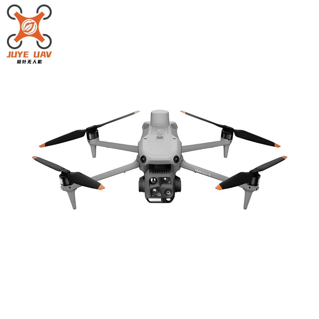
The above figure illustrates the overall system architecture for China UAV drone, showing the flow from multi-sensor input through three-level fusion to the memristor-based decision network.
3. Memristor-Based Deep Reinforcement Learning
To address the energy efficiency bottleneck of onboard computing for China UAV drone, we introduce a memristor-based processing-in-memory architecture to accelerate the inference of the deep Q-network. The core idea is to map the weights of fully connected layers to the programmable conductances of memristor crossbar arrays, enabling in-situ multiply-accumulate (MAC) operations with minimal energy consumption.
3.1 Memristor Device Model
We employ an improved HP memristor model with a threshold voltage mechanism to suppress unintended conductance drift. The equivalent resistance is:
$$
R(t) = R_{\text{on}} x(t) + R_{\text{off}} (1 – x(t))
$$
where $x(t) = \omega(t)/D$ is the normalized doping width. The state evolution is governed by:
$$
\frac{dx(t)}{dt} =
\begin{cases}
\frac{\mu_v R_{\text{on}}}{D^2} i(t) f(x), & |v(t)| > v_{\text{th}} \\
0, & |v(t)| \le v_{\text{th}}
\end{cases}
$$
with $f(x) = 1 – (2x-1)^{2p}$ (Joglekar window function). The threshold voltage $v_{\text{th}} = 0.5\,\text{V}$ prevents small voltage disturbances from altering the stored weight.
3.2 Weight Mapping and MAC Operation
For a fully connected layer with weight matrix $W$, each weight $w_{ij}$ is linearly quantized to a conductance range $[G_{\min}, G_{\max}]$:
$$
G_{ij} = G_{\min} + \frac{w_{ij} – w_{\min}}{w_{\max} – w_{\min}} (G_{\max} – G_{\min})
$$
To represent both positive and negative weights, we use a differential pair structure: $w_{ij} = k (G_{ij}^+ – G_{ij}^-)$. The input feature $x_i$ is encoded as a voltage $v_i$. The output current on the $j$-th bit-line is:
$$
I_j = \sum_i v_i (G_{ij}^+ – G_{ij}^-)
$$
This current is converted to a digital value via transimpedance amplifiers and ADCs, then passed through an activation function to produce Q-values.
3.3 Training Algorithm
We train the M-DQN using the standard DQN algorithm with experience replay and target network. The loss function is:
$$
L(\theta) = \mathbb{E}_{(s,a,r,s’) \sim D} \left[ \left( r + \gamma \max_{a’} Q(s’, a’; \theta^-) – Q(s,a;\theta) \right)^2 \right]
$$
The network parameters $\theta$ are updated by gradient descent, and the target network $\theta^-$ is periodically synchronized. During inference, the forward pass is executed on the memristor crossbar array, achieving energy-efficient real-time decision making for China UAV drone.
3.4 Improved APF Reward
The reward function integrates an improved artificial potential field to overcome local minima and oscillation. The attractive reward encourages moving toward the goal:
$$
R_{\text{att}}(t) = \eta_{\text{att}} \cdot d_{\text{goal}}(q)
$$
The repulsive reward penalizes proximity to obstacles:
$$
R_{\text{rep}}(t) = -\eta_{\text{rep}} \cdot \exp(-\gamma \cdot d_{\text{obs}}(q))
$$
Three improvements are incorporated: (1) smoothing function at the boundary of obstacle’s influence zone to avoid abrupt force changes; (2) dynamic virtual target point generation when a local minimum is detected:
$$
q_{\text{virtual}} = q_{\text{goal}} + \lambda \cdot \frac{q_{\text{goal}} – q}{\|q_{\text{goal}} – q\|} + \Delta_{\text{perturb}}
$$
(3) repulsive force direction optimization using a cosine factor to reduce opposite-direction components:
$$
F_{\text{rep}} = \eta_{\text{rep}} \left( \frac{1}{\rho} – \frac{1}{\rho_0} \right) \frac{\nabla \rho}{\rho^2} \cos\theta
$$
The final reward combines the APF dense reward with sparse terminal rewards (success: $+R_{\text{succ}}$, collision: $-R_{\text{coll}}$).
4. Experiments and Results
We conducted extensive simulations in a Python3.12.3 environment with PyTorch on a 2.20 GHz CPU and 16 GB RAM. The environment uses a standard grid map with static obstacles and four dynamic obstacles moving along predefined trajectories. The drone starts at (0,31) and the goal is at (31,0). The output is discrete action commands as described earlier.
4.1 Sensor Noise and RL Parameters
Table 1 lists the sensor noise parameters used in our simulations. Table 2 gives the reinforcement learning hyperparameters.
| Sensor | LiDAR | Vision | IMU | GPS |
|---|---|---|---|---|
| Noise std | 0.05 | 0.05 | 0.01 | 0.01 |
| Parameter | Value |
|---|---|
| Discount factor $\gamma$ | 0.99 |
| Learning rate $\alpha$ | 0.01 |
| Experience replay buffer size | 50000 |
| Target network update frequency | 400 |
| Initial exploration rate $\epsilon$ | 1.0 |
| Final exploration rate $\epsilon$ | 0.05 |
4.2 Perception Accuracy Comparison
We first compare the perception accuracy of single-modality (LiDAR only), dual-modal (LiDAR+Vision), and multimodal (LiDAR+Vision+IMU+GPS) under the same DQN decision layer. Table 3 and Figure 9 (conceptual) show the mean IoU and IoU variance.
| Perception Method | Mean IoU | IoU Variance |
|---|---|---|
| Single (LiDAR only) | 0.9092 | 0.003441 |
| Dual (LiDAR+Vision) | 0.9782 | 0.000355 |
| Multimodal (ours) | 0.9782 | 0.000354 |
Both dual-modal and multimodal achieve a mean IoU of 0.9782, which is 7.6% higher than the single-modality baseline. The variance is reduced by over 90%, demonstrating the effectiveness of multi-sensor complementarity for robust perception of China UAV drone.
4.3 Reward Function Ablation
We evaluate four reward function configurations: (a) Sparse target reward only; (b) Basic triple reward (target approach + collision penalty + step penalty); (c) Original APF hybrid reward; (d) Improved APF hybrid reward (our full method). Results are shown in Table 4, where the learning rate is 0.01, and all other hyperparameters are the same.
| Reward Type | Success Rate | Avg Path Length | Local Min. Occurrence | Avg Converg. Episodes |
|---|---|---|---|---|
| Sparse target only | 0% | 128.00 | 92.0% | 800.0 |
| Basic triple | 80% | 49.89 | 20.0% | 233.3 |
| Original APF | 100% | 31.18 | 0.0% | 283.3 |
| Improved APF (ours) | 100% | 30.31 | 0.0% | 200.0 |
The improved APF reward achieves a 100% success rate with the shortest average path length (30.31 steps) and converges in only 200 episodes, confirming the effectiveness of the proposed smoothing, virtual target, and force direction optimization.
4.4 Memristor DQN Performance in Static and Dynamic Environments
We compare traditional DQN (simulated with standard digital circuits), memristor DQN (M-DQN), and two baseline algorithms (ICVTLBO from [26] and DDQN-3D from [27]) in both static and dynamic environments. The memristor parameters are given in Table 5.
| Parameter | Value |
|---|---|
| Minimum resistance $R_{\text{on}}$ | $10^4\,\Omega$ |
| Maximum resistance $R_{\text{off}}$ | $10^6\,\Omega$ |
| Initial memristance ratio | 0.1 |
| Linear drift coefficient | $10^{-14}\,\text{m}^2\text{s}^{-1}\text{V}^{-1}$ |
| Memristor length | 10 nm |
| Threshold voltage $v_{\text{th}}$ | 0.5 V |
| Window function parameter $p$ | 5 |
| Operating frequency | 6 Hz |
Static Environment: Results are shown in Table 6.
| Algorithm | Success Rate | Path Length | Energy/Step ($\mu$J) | Inference Time (ms) |
|---|---|---|---|---|
| Traditional DQN | 100% | 62.00 | 62 | 0.0205 |
| M-DQN (ours) | 98.3% | 68.96 | 5.516 | 0.0056 |
| ICVTLBO [26] | 100% | 62.00 | 8664 | 246.3571 |
M-DQN achieves 98.3% success rate, slightly lower than traditional DQN due to non-ideal memristor characteristics, but the energy per step is reduced by 91.1% (from 62 $\mu$J to 5.516 $\mu$J) and inference time is 3.7 times faster. ICVTLBO has extremely high energy and inference time.
Dynamic Environment (4 moving obstacles as per Table 7):
| Obstacle | Start Pos. | Direction | Speed |
|---|---|---|---|
| $m_1$ | (3,0) | (0,1) | 1 unit/s |
| $m_2$ | (31,28) | (-1,0) | 1 unit/s |
| $m_3$ | (15,31) | (0,-1) | 1 unit/s |
| $m_4$ | (31,4) | (-1,0) | 1 unit/s |
Results are shown in Table 8.
| Algorithm | Success Rate | Path Length | Energy ($\mu$J) | Inference Time (ms) |
|---|---|---|---|---|
| Traditional DQN | 94.7% | 74.2 | 90.1 | 0.04 |
| M-DQN (ours) | 100% | 63.1 | 76.0 | 0.09 |
| DDQN-3D [27] | 98.7% | 75.9 | 92.1 | 0.19 |
In the dynamic environment, our M-DQN achieves 100% success rate, 15.0% shorter path length, and 15.7% lower energy consumption compared to traditional DQN. Compared to DDQN-3D, M-DQN is superior in all metrics except inference time, which is still at the sub-millisecond level. The results demonstrate that our memristor-based approach provides excellent performance for real-time obstacle avoidance of China UAV drone in dynamic scenarios.
4.5 Sensitivity Analysis on Learning Rate
We investigate the effect of learning rate $\alpha$ on our multimodal M-DQN algorithm in both static and dynamic environments. Table 9 summarizes the results.
| Learning Rate $\alpha$ | Static Environment | Dynamic Environment | ||||
|---|---|---|---|---|---|---|
| Success Rate | Avg Energy ($\mu$J) | Converg. Episodes | Success Rate | Avg Energy ($\mu$J) | Converg. Episodes | |
| 0.001 | 88.0% | 9.346 | 716.7 | 100.0% | 5.326 | 516.8 |
| 0.01 | 100.0% | 5.165 | 666.7 | 100.0% | 2.590 | 733.3 |
| 0.1 | 0.0% | 20.480 | 1000.0 | 0.0% | 3.290 | 1000.0 |
A learning rate of 0.01 yields the best overall performance: 100% success in both environments, lowest energy consumption, and reasonable convergence speed. The rate 0.001 leads to slower convergence and a local minimum issue in the static environment, while 0.1 causes gradient explosion and complete failure. This sensitivity study provides guidance for deploying our method on actual China UAV drone platforms.
5. Conclusion
We have presented a comprehensive obstacle avoidance strategy for China UAV drone that tightly integrates multimodal fusion perception and memristor-based deep reinforcement learning. The three-level adaptive fusion framework effectively mitigates single-sensor weaknesses, achieving high perception accuracy (mean IoU 0.9782) and robustness. The improved APF reward resolves local minima and trajectory oscillation, leading to 100% success rate and fast convergence (200 episodes). The memristor DQN reduces per-step energy consumption by over 91% in static environments and 15.7% in dynamic environments while maintaining a high success rate (100% in dynamic benchmarks). Our work demonstrates that the combination of multimodal perception and in-memory computing provides a practical and energy-efficient solution for autonomous navigation of China UAV drone in complex, dynamic, and resource-constrained operational settings. Future work will focus on extending the method to continuous control tasks, multi-UAV coordination, and extreme weather conditions, further advancing the capabilities of China UAV drone in real-world applications.