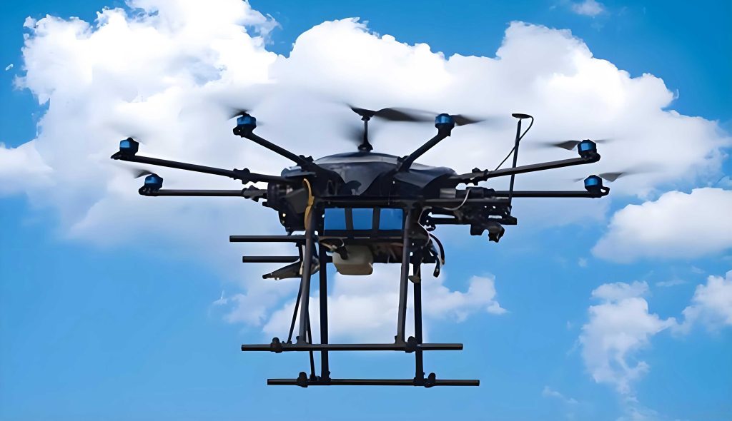
The evolution of modern warfare, characterized by high dynamics and intense confrontation, has driven a paradigm shift in tactical operations. The emergence of sophisticated missile defense technologies has necessitated the development of more resilient and effective offensive systems. In this complex and demanding battlespace, a novel combat paradigm has taken center stage: cooperative swarm operations for aerial platforms. For UAV drones, this mode represents the future of aerial combat, leveraging the synergistic potential of multiple, heterogeneous units to achieve objectives unattainable by single platforms. The effectiveness of these UAV drone swarms is not merely an additive function but a complex emergent property, making its accurate assessment a critical and challenging endeavor. Precise evaluation of combat effectiveness directly influences the success of operational plans. Therefore, to optimize mission outcomes and enhance success rates, it is imperative to construct evaluation models that closely mirror actual combat conditions.
UAV drones operating in collaborative swarms present a new frontier in information-centric warfare. To harness and elevate the coordinated combat power of UAV drone clusters, we must account for a multitude of influencing factors. This requires quantifying these factors, establishing corresponding computational frameworks, and exploring their impact on the overall system效能. This process forms the foundation for improving, optimizing, and refining the models used to assess the operational效能 of UAV drones. The factors affecting swarm effectiveness are numerous, with many possessing inherent uncertainties. The correlations between these factors and the relative importance of each can significantly influence model accuracy. Global sensitivity analysis serves as a vital tool for identifying key parameters and quantifying their interactions, measuring the influence of individual and combined factors on the target function. Consequently, applying such analysis to uncover the most significant factors affecting UAV drone swarm effectiveness, while accounting for their uncertainties, holds substantial research value for enhancing model precision.
This article focuses on establishing a fundamental cooperative combat effectiveness model for UAV drones based on the ADC framework, developing a corresponding importance measure model, and conducting a sensitivity analysis on relevant parameters to obtain a sensitivity ranking. This analysis helps identify the degree to which each factor influences overall效能, thereby improving model accuracy. The resulting sensitivity sequence offers rapid identification capability, pinpointing key parameters that potentially affect system reliability and guiding改进s in system design.
Fundamental Model for UAV Drones Cooperative Combat Effectiveness
The foundational model for assessing the cooperative combat effectiveness of UAV drones must integrate the myriad practical factors affecting a swarm’s performance. These include the battlefield environment, command personnel proficiency, inherent combat capabilities, and the individual performance metrics of the UAV drones themselves. Establishing a model that closely approximates real-world conditions, while simplifying the evaluation指标体系 for tractability, is essential. Unlike evaluating a single UAV drone or simple cooperation between identical units, a swarm model must account for the synergistic effects of heterogeneous UAV drones working in concert, necessitating a simplified yet representative framework. Probability models are generally more suitable than deterministic ones for assessing the complex效能 of UAV drone协同作战, as they can accommodate various uncertainties within the indicators, ensuring comprehensiveness and accuracy.
The ADC Framework and Utility Function Method
In 1965, the US Weapon System Effectiveness Industry Advisory Committee (WSEIAC) proposed the ADC method for effectiveness evaluation. The core formula is:
$$E = A \times D \times C$$
where \(E\) represents the overall system effectiveness, \(A\) denotes availability (the probability the system is ready when needed), \(D\) represents dependability (the probability it will perform as required during a mission), and \(C\) signifies capability (the system’s performance level given it is functioning). The ADC method holistically reflects overall效能 by capturing the interplay between reliability, supportability, and inherent capability, making it widely applicable for large weapon systems like UAV drone swarms.
For applying the ADC method to UAV drones, effectiveness evaluation models are typically built using either dimensional or probabilistic approaches. A more integrated method, the Utility Function Method, is employed here. This method processes dimensional indicators via utility functions and divides probabilistic indicators into qualitative and quantitative types. Quantitative indicators are handled probabilistically, while qualitative ones are addressed using scaling methods. The availability vector \(A\) is generated through ratio calculation. Subsequently, the dependability matrix \(D\) can be derived using methods like exponential distributions for reliability indicators. Thus, the Utility Function Method constitutes a comprehensive effectiveness evaluation model.
Traditional Model for UAV Drones Cooperative Combat Effectiveness
Let \(E\) represent the cooperative combat capability of a UAV drone swarm. The mathematical model is established as:
$$E = \epsilon_1 E_{GZ} + \epsilon_2 E_{TX} + \epsilon_3 E_{CH} + \epsilon_4 E_{DJ} + \epsilon_5 E_{ZD} – \theta_s$$
where \(E_{GZ}\), \(E_{TX}\), \(E_{CH}\), \(E_{DJ}\), and \(E_{ZD}\) denote协同感知, communication, planning, strike, and teaming capabilities, respectively. The weights for each subsystem are represented by \(\epsilon_i\) (for \(i=1,2,…,5\)), and \(\theta_s\) is a coefficient representing效能 loss.
1.协同感知 Capability (\(E_{GZ}\)):
For a single UAV drone (\(E_{GZW}\)):
$$E_{GZW} = \eta_1 E_{LD} + \eta_2 E_{GD} + \eta_3 E_{EZ}$$
where \(E_{LD}\), \(E_{GD}\), and \(E_{EZ}\) represent radar detection, electro-optical detection, and electronic reconnaissance capabilities. \(\eta_1, \eta_2, \eta_3\) are their respective weights.
For a swarm of \(m\) UAV drones, the cooperative感知 capability is the superposition:
$$E_{GZ} = \sum_{j=1}^{m} E_{GZW,j}$$
where \(E_{GZW,j}\) is the感知 capability of the \(j\)-th UAV drone.
2.协同Communication Capability (\(E_{TX}\)):
For a single UAV drone (\(E_{TXW}\)):
$$E_{TXW} = \eta_4 E_{P} + \eta_5 E_{Q} + \eta_6 E_{C}$$
where \(E_{P}\), \(E_{Q}\), and \(E_{C}\) denote timeliness, effective system capacity, and node connectivity.
For the swarm:
$$E_{TX} = \sum_{j=1}^{m} E_{TXW,j}$$
3.协同Planning Capability (\(E_{CH}\)):
For a single UAV drone (\(E_{CHW}\)):
$$E_{CHW} = \eta_7 E_{gh} + \eta_8 E_{kc} + \eta_9 E_{jc}$$
where \(E_{gh}\), \(E_{kc}\), and \(E_{jc}\) represent cooperative mission planning, cooperative control relations, and dynamic real-time decision-making.
For the swarm:
$$E_{CH} = \sum_{j=1}^{m} E_{CHW,j}$$
4.协同Strike Capability (\(E_{DJ}\)):
The model is described as:
$$E_{DJ} = \eta_{10} \frac{\sum_{j=1}^{m} E_{GJW,j}}{m} + \eta_{11} \sum_{j=1}^{m} E_{GBW,j}$$
where \(E_{GJW,j}\) and \(E_{GBW,j}\) are the attack and evasion capabilities of the \(j\)-th UAV drone, and \(E_{CJW,j}\) is its cooperative attack capability. \(\eta_{10}\) and \(\eta_{11}\) are weights.
5.协同Teaming Capability (\(E_{ZD}\)):
Comprising flight performance, survivability, and availability:
$$E_{ZD} = \eta_{12} \frac{\sum_{j=1}^{m} E_{FXW,j}}{m} + \eta_{13} \frac{\sum_{j=1}^{m} E_{KYW,j}}{m} + \eta_{14} \frac{\sum_{j=1}^{m} E_{SCW,j}}{m}$$
where \(E_{FXW,j}\), \(E_{KYW,j}\), and \(E_{SCW,j}\) are the flight performance, availability, and survivability of the \(j\)-th UAV drone. \(\eta_{12}, \eta_{13}, \eta_{14}\) are weights.
To illustrate, consider two types of UAV drones, Type A and Type B, with different capability profiles. The weights for the system and sub-capabilities, often derived from expert scoring, are presented in the tables below.
| Capability Indicator | Type A UAV Drone | Type B UAV Drone |
|---|---|---|
| Radar Detection \(E_{LD}\) | 0.7267 | 0.0000 |
| Electro-Optical Detection \(E_{GD}\) | 1.0267 | 1.0267 |
| Electronic Reconnaissance \(E_{EZ}\) | 0.0000 | 1.3661 |
| Timeliness \(E_{P}\) | 0.3000 | 0.3000 |
| Effective System Capacity \(E_{Q}\) | 0.2000 | 0.2000 |
| Node Connectivity \(E_{C}\) | 0.4250 | 0.4250 |
| Cooperative Mission Planning \(E_{gh}\) | 0.5333 | 0.5333 |
| Cooperative Control Relations \(E_{kc}\) | 0.3300 | 0.3300 |
| Dynamic Real-Time Decision \(E_{jc}\) | 0.3300 | 0.3300 |
| Attack Capability \(E_{GJW}\) | 0.3900 | 0.8731 |
| Evasion Capability \(E_{GBW}\) | 0.2000 | 0.2000 |
| Flight Performance \(E_{FXW}\) | 0.2807 | 0.2574 |
| Availability \(E_{KYW}\) | 0.8400 | 0.8400 |
| Survivability \(E_{SCW}\) | 1.1672 | 1.1672 |
| Weight Symbol | Value |
|---|---|
| \(\epsilon_1\) | 0.156 |
| \(\epsilon_2\) | 0.193 |
| \(\epsilon_3\) | 0.192 |
| \(\epsilon_4\) | 0.211 |
| \(\epsilon_5\) | 0.248 |
| \(\eta_1\) | 0.689 |
| \(\eta_2\) | 0.188 |
| \(\eta_3\) | 0.123 |
| \(\eta_4\) | 0.449 |
| \(\eta_5\) | 0.231 |
| \(\eta_6\) | 0.320 |
| \(\eta_7\) | 0.367 |
| \(\eta_8\) | 0.260 |
| \(\eta_9\) | 0.373 |
| \(\eta_{10}\) | 0.665 |
| \(\eta_{11}\) | 0.335 |
| \(\eta_{12}\) | 0.533 |
| \(\eta_{13}\) | 0.272 |
| \(\eta_{14}\) | 0.195 |
Importance Measure Model and Sensitivity Analysis
Importance Measure Model
The overall combat effectiveness of the UAV drone swarm responds differently to the randomness of various parameters. Identifying which random variable parameters most significantly influence the improvement of overall effectiveness is crucial for refining the study of UAV drone swarm协同作战, aiming to maximize effectiveness while ensuring operational safety. By simulating the aforementioned mathematical model, we can analyze the response of the overall effectiveness \(E\) to the randomness of each parameter—essentially conducting a sensitivity analysis on the model’s效能. Studying the sensitivity to the mean of each random parameter can be defined as the partial derivative of the overall effectiveness \(E\) with respect to the mean of each random parameter, expressed as \(\partial E / \partial \mu_{E_i}\), where \(\mu_{E_i}\) is the mean of the \(i\)-th random variable.
Conducting this reliability sensitivity analysis requires treating all capability indicators of the UAV drones as independent normal random variables. The distribution information for these variables is summarized below.
| Random Variable | Mean Value | Coefficient of Variation | Distribution Type |
|---|---|---|---|
| \(E_{LD}\) | 0.7267 | 0.1 | Normal |
| \(E_{GD}\) | 1.0267 | 0.1 | Normal |
| \(E_{EZ}\) | 0.0000 | 0.1 | Normal |
| \(E_{P}\) | 0.3000 | 0.1 | Normal |
| \(E_{Q}\) | 0.2000 | 0.1 | Normal |
| \(E_{C}\) | 0.4250 | 0.1 | Normal |
| \(E_{gh}\) | 0.5333 | 0.1 | Normal |
| \(E_{kc}\) | 0.3300 | 0.1 | Normal |
| \(E_{jc}\) | 0.3300 | 0.1 | Normal |
| \(E_{GJW}\) | 0.3900 | 0.1 | Normal |
| \(E_{GBW}\) | 0.2000 | 0.1 | Normal |
| \(E_{FXW}\) | 0.2807 | 0.1 | Normal |
| \(E_{KYW}\) | 0.8400 | 0.1 | Normal |
| \(E_{SCW}\) | 1.1672 | 0.1 | Normal |
| Random Variable | Mean Value | Coefficient of Variation | Distribution Type |
|---|---|---|---|
| \(E_{LD}\) | 0.0000 | 0.1 | Normal |
| \(E_{GD}\) | 1.0267 | 0.1 | Normal |
| \(E_{EZ}\) | 1.3661 | 0.1 | Normal |
| \(E_{P}\) | 0.3000 | 0.1 | Normal |
| \(E_{Q}\) | 0.2000 | 0.1 | Normal |
| \(E_{C}\) | 0.4250 | 0.1 | Normal |
| \(E_{gh}\) | 0.5333 | 0.1 | Normal |
| \(E_{kc}\) | 0.3300 | 0.1 | Normal |
| \(E_{jc}\) | 0.3300 | 0.1 | Normal |
| \(E_{GJW}\) | 0.8731 | 0.1 | Normal |
| \(E_{GBW}\) | 0.2000 | 0.1 | Normal |
| \(E_{FXW}\) | 0.2574 | 0.1 | Normal |
| \(E_{KYW}\) | 0.8400 | 0.1 | Normal |
| \(E_{SCW}\) | 1.1672 | 0.1 | Normal |
For a combat scenario involving 4 Type A and 4 Type B UAV drones, we perform a sensitivity analysis on the model’s effectiveness. Using area-based methods (or global sensitivity methods like Sobol), the sensitivity of each random variable can be calculated. The results, summarized in the table below, indicate that radar detection capability, cooperative mission planning, and attack capability exhibit the highest sensitivity. Therefore, variations in these three capabilities during operations have the most significant impact on the overall协同作战效能 of the UAV drone swarm.
| Capability Indicator | Sensitivity for Type A UAV Drones | Sensitivity for Type B UAV Drones |
|---|---|---|
| Radar Detection \(E_{LD}\) | 0.1718 | 0.0000 |
| Electro-Optical Detection \(E_{GD}\) | 0.0551 | 0.0437 |
| Electronic Reconnaissance \(E_{EZ}\) | 0.0000 | 0.0483 |
| Timeliness \(E_{P}\) | 0.0426 | 0.0467 |
| Effective System Capacity \(E_{Q}\) | 0.0140 | 0.0150 |
| Node Connectivity \(E_{C}\) | 0.0505 | 0.0442 |
| Cooperative Mission Planning \(E_{gh}\) | 0.0676 | 0.0656 |
| Cooperative Control Relations \(E_{kc}\) | 0.0280 | 0.0243 |
| Dynamic Real-Time Decision \(E_{jc}\) | 0.0376 | 0.0389 |
| Attack Capability \(E_{GJW}\) | 0.0918 | 0.2750 |
| Evasion Capability \(E_{GBW}\) | 0.0027 | 0.0027 |
| Flight Performance \(E_{FXW}\) | 0.0102 | 0.0112 |
| Availability \(E_{KYW}\) | 0.0104 | 0.0131 |
| Survivability \(E_{SCW}\) | 1.4815e-05 | 1.5963e-05 |
Availability (A) Analysis
The vector \(A\) represents the state of the UAV drone formation before a combat mission begins. Assume a mission deploys \(n\) Type A and \(m\) Type B UAV drones. Pre-mission checks determine that \(k\) UAV drones are in an operational state, and this number must be sufficient to commence the mission, considering constraints like required minimum force.
The availability for a single UAV drone of type \(i\) is given by:
$$a_i = \frac{MTBF_i}{MTBF_i + MTTR_i}$$
where \(MTBF_i\) is the Mean Time Between Failures and \(MTTR_i\) is the Mean Time To Repair.
The system state calculation involves enumerating all possible combinations of operational and failed UAV drones subject to the constraint of having at least \(k\) operational units. This process yields the availability vector \(A\), where each element \(A_j\) is the probability of the system being in state \(j\) at mission start.
Dependability (D) Analysis
The dependability matrix \(D(t)\) represents the probability of the system transitioning between states during the mission, given it starts in a specific state. For a system with \(n\) states, \(D(t)\) is an \(n \times n\) matrix:
$$
D(t) =
\begin{bmatrix}
d_{11}(t) & d_{12}(t) & \cdots & d_{1n}(t) \\
d_{21}(t) & d_{22}(t) & \cdots & d_{2n}(t) \\
\vdots & \vdots & \ddots & \vdots \\
d_{n1}(t) & d_{n2}(t) & \cdots & d_{nn}(t)
\end{bmatrix}
$$
where \(d_{ij}(t)\) is the probability of transitioning from state \(i\) to state \(j\) by time \(t\). For non-repairable systems during a mission (a common assumption for UAV drones), the matrix becomes upper triangular, as the system can only degrade.
To compute \(d_{ij}(t)\), we need the reliability function for each UAV drone type. The reliability at time \(t\) is:
$$R_i(t) = e^{-\lambda_i t}, \quad \text{where } \lambda_i = 1/MTBF_i$$
However, the operational state of a UAV drone also depends on its survivability \(S_{ur}\), which is influenced by factors like Radar Cross Section (RCS), wing area \(S\), attack length \(L\), cruise speed \(V\), and maximum payload \(W\). A simplified, normalized model can be:
$$S_{ur} = 0.25 \cdot RCS + 0.15 \cdot S + 0.1 \cdot L + 0.3 \cdot V + 0.2 \cdot W$$
The effective “operational availability” during a mission for a UAV drone of type \(i\) at time \(t\) can then be modeled as:
$$U_i(t) = R_i(t) \cdot S_{ur,i}$$
The transition probabilities \(d_{ij}(t)\) are computed based on combinations of \(U_i(t)\) for surviving UAV drones and \((1-U_i(t))\) for failing ones, considering the specific state definitions. If the mission duration exceeds the maximum endurance \(T_{end,i}\) of a UAV drone type, its \(U_i(t)\) becomes 0 for \(t > T_{end,i}\). The final dependability matrix for a mission of duration \(T\) might be a product of matrices for different time segments:
$$D = D(t_1) \times D(t_2) \times … \times D(t_p)$$
where each segment corresponds to a period before a specific UAV drone type reaches its endurance limit.
Case Study and Simulation Analysis
This section presents a simulation to demonstrate the application of the ADC model and sensitivity analysis for a UAV drone协同作战 system.
Scenario: A mission is launched with a total of 4 UAV drones, which can be a mix of Type A (reconnaissance-strike) and Type B (electronic warfare-strike). The mission requires at least 3 UAV drones to be fully operational. The mission duration is set to 1 hour, and UAV drones are assumed to be non-repairable during the mission. We evaluate five possible compositions (schemes):
- 1 Type A + 3 Type B UAV Drones
- 2 Type A + 2 Type B UAV Drones
- 3 Type A + 1 Type B UAV Drone
- 4 Type A UAV Drones
- 4 Type B UAV Drones
The performance parameters for the two types of UAV drones are listed below.
| Performance Indicator | Type A UAV Drone | Type B UAV Drone |
|---|---|---|
| SAR Radar | 1 | 0 |
| ESM Equipment | 1 | 1 |
| EO/IR Detection | 0 | 1 |
| Attack Payload | 4 | 9 |
| MTBF (hours) | 70 | 50 |
| MTTR (hours) | 1 | 1 |
| RCS (m²) | 0.80 | 0.93 |
| Wing Area S (m²) | 63.2 | 58.3 |
| Length L (m) | 11.63 | 8.13 |
| Max Cruise Speed V (m/s) | 60 | 69 |
| Max Payload W (kg) | 2 | 1.5 |
| Max Endurance (hours) | 8 | 7 |
Analysis for Scheme 1 (1A+3B):
The system states are defined based on the number of operational UAV drones. The availability vector \(A\) is computed based on the pre-mission reliability. The dependability matrix \(D(t)\) is constructed considering the reliability functions \(R_A(t)\) and \(R_B(t)\), and the survivability factors. The capability vector \(C\) is calculated using the cooperative combat model from Section 1.3, populated with the appropriate capability values for the surviving UAV drones in each state.
The overall effectiveness \(E(t) = A \cdot D(t) \cdot C\) is then computed as a function of mission time. The result shows that effectiveness gradually decreases over time. A sharp drop occurs after 6 hours when the Type B UAV drones reach their endurance limit (\(T_{end,B}=7h\)), and effectiveness falls to zero after 7 hours when all Type B UAV drones are no longer operational.
Furthermore, a Sobol global sensitivity analysis can be performed on parameters like RCS, wing area, length, and cruise speed for the UAV drones in this scheme. The results would typically show that parameters like the RCS of Type B UAV drones and their maximum cruise speed have the highest Sobol indices (total-effect), indicating they are the most influential factors affecting作战效能 variability and should be key design considerations.
Comparison of All Schemes:
By calculating \(E(t)\) for each of the five schemes over the mission duration, we can compare their effectiveness profiles. The analysis might reveal, for instance, that Scheme 4 (all Type A) has the highest effectiveness for missions shorter than approximately 3.5 hours, while Scheme 5 (all Type B) becomes superior for longer missions due to its higher payload or other capability factors, despite its shorter endurance. This comparison aids in selecting the optimal UAV drone composition based on the expected mission duration, a crucial decision for commanders employing UAV drone swarms.
Conclusion and Future Directions
This article has established a comprehensive framework for evaluating the cooperative combat effectiveness of UAV drone swarms based on the ADC model. The framework integrates key效能 indicators into a mathematical model for UAV drone协同作战能力, accounting for协同感知, communication, planning, strike, and teaming capabilities. We further developed an importance measure model and conducted parameter sensitivity analysis, identifying which random variables—such as radar detection, cooperative mission planning, and attack capabilities—most significantly influence the overall效能 of the UAV drone swarm. This insight is vital for prioritizing design改进s and operational focus to maximize effectiveness under uncertainty.
The analysis of availability and dependability provides the probabilistic foundation for the model, crucial for assessing UAV drone swarm performance in realistic, stochastic environments. The case study demonstrated the practical application of the model, showing how effectiveness evolves with mission time and how different compositions of heterogeneous UAV drones compare, enabling data-driven force packaging decisions.
Future research directions for UAV drone swarm effectiveness modeling are vast. Integration with more advanced global sensitivity analysis methods, such as variance-based or metamodel-based techniques, could provide deeper insights into high-order interactions between parameters. The model can be extended to incorporate dynamic adversarial interactions, learning and adaptation capabilities of UAV drones, and more sophisticated communications and networking models. Furthermore, coupling this effectiveness model with mission planning and real-time control algorithms will be essential for developing truly autonomous and effective UAV drone swarms capable of operating in the complex, high-threat environments of future battlefields. The continuous refinement of such models is paramount for maintaining tactical and technological superiority in an era defined by collaborative autonomous systems like UAV drones.