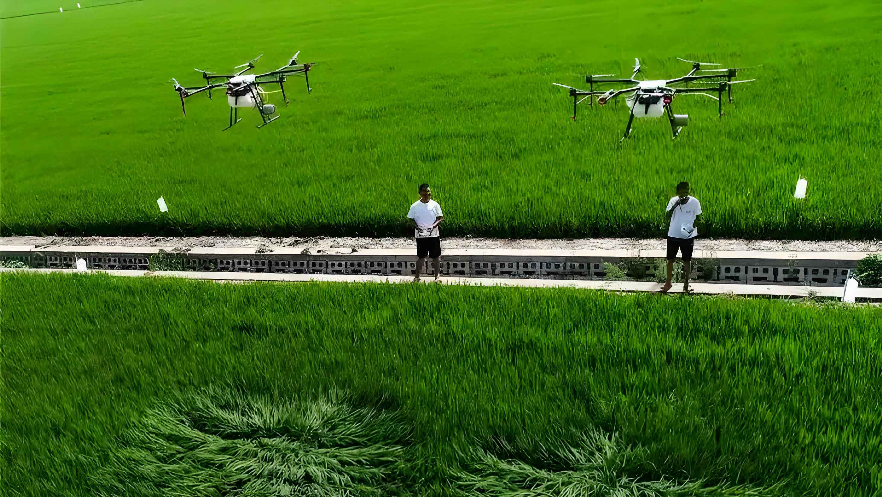
In recent years, the rapid advancement of technology has led to the widespread application of agricultural UAVs in agricultural production. These UAVs have significantly improved work efficiency and reduced labor and material consumption. With the growing demand driven by large-scale farming, the market for agricultural UAVs has matured, transitioning from manual operation to intelligent systems. However, existing spraying methods for agricultural UAVs often rely on relatively crude operations, heavily dependent on manual control by pilots or pre-set programs. This reliance on human judgment frequently results in uneven pesticide concentrations, missed sprays, or overlapping applications, particularly during obstacle avoidance, deceleration, or row-changing maneuvers. Such issues can lead to over-spraying, crop damage, and negatively impact plant growth. To ensure the operational quality of agricultural UAVs, there is a pressing need to optimize their spraying systems. The control of pesticide mixing ratios and flow rates remains a challenge, and achieving intelligent control of the spraying system is an urgent problem to address. In this article, I present a comprehensive design for an intelligent spraying system tailored for agricultural UAVs, aimed at enhancing precision and efficiency in crop protection.
The intelligent spraying system I propose consists of three core units: the Intelligent Dosing Unit, the Precision Spraying Unit, and the Intelligent Monitoring Unit. These units work in tandem, leveraging smart algorithms for real-time optimization during flight operations. This integrated approach addresses the shortcomings of traditional methods by enabling automated pesticide mixing, precise flow control, and comprehensive system monitoring. Throughout this discussion, I will delve into the hardware design, control mechanisms, and algorithmic foundations that make this system a transformative tool for modern agriculture. By incorporating advanced technologies, this system not only boosts the performance of agricultural UAVs but also promotes sustainable farming practices through reduced chemical usage and minimized environmental impact.
Intelligent Dosing Unit: Automated Pesticide Preparation
The Intelligent Dosing Unit is responsible for high-precision pesticide mixing and blending. It ensures that pesticides and water are combined in accurate ratios according to crop requirements, thereby optimizing efficacy and reducing waste. This unit comprises several key components: pesticide tanks, water tanks, control units, a blending unit, a mixing unit, and a spray tank. The process begins with control unit 1 monitoring the liquid level and concentration in the pesticide tank, while control unit 2 tracks the water level in the water tank. Based on predefined operational needs, these control units regulate the flow of pesticide and water to achieve the desired mixing ratio. The pre-mixed solution is then transferred to a blending area, where initial homogenization occurs. For pesticides that require thorough dissolution or agitation, the mixture is further processed in a mixing unit equipped with an electric stirrer. Finally, a concentration sensor validates the mixture before it is pumped into the spray tank for deployment.
To quantify the mixing process, we can model the concentration dynamics using differential equations. Let \( C_p \) be the concentration of pesticide in the mixture, \( V \) the total volume, and \( Q_p \) and \( Q_w \) the flow rates of pesticide and water, respectively. The rate of change of pesticide mass is given by:
$$ \frac{d(C_p V)}{dt} = Q_p C_{p0} – (Q_p + Q_w) C_p $$
where \( C_{p0} \) is the initial concentration in the pesticide tank. Assuming constant volume \( V \) during mixing, this simplifies to:
$$ V \frac{dC_p}{dt} = Q_p (C_{p0} – C_p) – Q_w C_p $$
By controlling \( Q_p \) and \( Q_w \) via feedback from concentration sensors, we can achieve a target concentration \( C_{target} \). The control law can be expressed as:
$$ Q_p = k_p (C_{target} – C_p) + k_i \int (C_{target} – C_p) dt $$
where \( k_p \) and \( k_i \) are proportional and integral gains, respectively. This ensures rapid convergence to the desired ratio, minimizing errors. The following table summarizes the key parameters and their typical ranges in the Intelligent Dosing Unit:
| Parameter | Description | Typical Range |
|---|---|---|
| Pesticide Flow Rate (\( Q_p \)) | Flow rate of pesticide from tank | 0.1–5 L/min |
| Water Flow Rate (\( Q_w \)) | Flow rate of water from tank | 1–20 L/min |
| Mixing Volume (\( V \)) | Total volume in blending unit | 10–100 L |
| Concentration Error (\( \Delta C \)) | Deviation from target concentration | ±0.5% |
| Response Time (\( t_r \)) | Time to reach target concentration | < 30 seconds |
This unit eliminates the guesswork in manual dosing, ensuring consistent pesticide formulations that enhance crop safety and effectiveness. By integrating such precision, agricultural UAVs can adapt to varying field conditions, such as different pest pressures or crop growth stages, thereby optimizing resource use.
Precision Spraying Unit: Real-Time Flow and Pressure Control
The Precision Spraying Unit governs the actual spraying operation during flight, enabling accurate application of pesticides based on real-time data. It consists of a spraying CPU, a frequency conversion unit, a pump unit, and adjustable nozzle units. The spraying CPU sends control signals to the frequency conversion unit, which modulates the pump’s operation to regulate flow rate and pressure. The pump then delivers the pesticide mixture to the nozzles, which can be independently controlled for spray angle and pattern. Feedback mechanisms include flow sensors and pressure transducers that relay data back to the spraying CPU, allowing for closed-loop control.
The dynamics of the spraying process can be described using fluid mechanics principles. The flow rate \( Q \) through a nozzle is related to the pressure \( P \) by:
$$ Q = C_d A \sqrt{\frac{2P}{\rho}} $$
where \( C_d \) is the discharge coefficient, \( A \) is the nozzle area, and \( \rho \) is the fluid density. To maintain a desired flow rate \( Q_{des} \) as the agricultural UAV moves, we adjust the pump speed via the frequency conversion unit. The pump’s performance can be modeled as:
$$ P = k \omega^2 – R Q^2 $$
where \( \omega \) is the pump rotational speed, \( k \) is a constant, and \( R \) represents hydraulic resistance. Combining these equations, we derive a control law for the spraying CPU:
$$ \omega = \sqrt{\frac{P_{des} + R Q_{des}^2}{k}} $$
with \( P_{des} \) calculated from \( Q_{des} \) using the nozzle equation. This ensures consistent spray deposition even when the UAV changes speed or altitude. The following table outlines the operational parameters for the Precision Spraying Unit:
| Parameter | Description | Typical Value |
|---|---|---|
| Nozzle Flow Rate (\( Q \)) | Flow rate per nozzle | 0.5–2 L/min |
| Spray Pressure (\( P \)) | Operating pressure | 0.2–0.8 MPa |
| Nozzle Count | Number of adjustable nozzles | 4–8 per UAV |
| Control Frequency (\( f \)) | Update rate of spraying CPU | 100 Hz |
| Spray Swath Width | Coverage width per pass | 3–10 meters |
By leveraging this unit, agricultural UAVs can achieve variable-rate spraying, where pesticide application is modulated based on crop density or pest maps. This precision reduces chemical runoff and promotes targeted treatment, aligning with sustainable agriculture goals. The integration of feedback loops allows the system to compensate for disturbances like wind or terrain variations, ensuring uniform coverage.
Intelligent Monitoring Unit: Data Integration and Algorithmic Optimization
The Intelligent Monitoring Unit serves as the brain of the system, collecting and analyzing data from various sources to optimize spraying operations in real time. It includes a monitoring CPU, flight data acquisition units, spraying data acquisition units, external environment sensors, and an intelligent algorithm module. The monitoring CPU gathers data on UAV flight parameters (e.g., speed, altitude, attitude), spraying metrics (e.g., flow rates, pressure), and environmental conditions (e.g., wind speed, temperature, humidity). These data streams are processed using convolutional neural networks (CNNs) or other machine learning algorithms to generate optimization commands, which are then fed back to the spraying CPU for adjustments.
The optimization problem can be formulated as minimizing a cost function \( J \) that accounts for spraying efficacy and resource usage:
$$ J = \alpha \sum_{i=1}^{N} (D_i – D_{target})^2 + \beta \int Q(t) dt + \gamma \int E(t) dt $$
where \( D_i \) is the deposition density at location \( i \), \( D_{target} \) is the desired deposition, \( Q(t) \) is the flow rate over time, \( E(t) \) represents environmental factors like drift, and \( \alpha, \beta, \gamma \) are weighting coefficients. The CNN processes input data \( \mathbf{X} \) (e.g., sensor readings) to predict optimal control actions \( \mathbf{U} \):
$$ \mathbf{U} = f_{CNN}(\mathbf{X}; \theta) $$
with parameters \( \theta \) learned from historical data. Training involves minimizing the mean squared error between predicted and ideal actions. For instance, the network might learn to adjust nozzle settings based on wind patterns to reduce drift. The following table summarizes key data inputs and outputs for the Intelligent Monitoring Unit:
| Data Type | Source | Sampling Rate | Optimization Output |
|---|---|---|---|
| Flight Speed | GPS/IMU sensors | 50 Hz | Adjusted UAV velocity |
| Spray Flow Rate | Flow meters | 20 Hz | Modulated pump speed |
| Wind Speed | Anemometers | 10 Hz | Nozzle angle correction |
| Crop Health Index | Multispectral cameras | 5 Hz | Variable-rate spraying map |
| Battery Level | Power management system | 1 Hz | Optimized flight path |
This unit enables adaptive spraying, where the agricultural UAV responds dynamically to field conditions. For example, if the system detects an area with higher pest infestation, it can increase pesticide dosage locally. The use of CNNs allows for pattern recognition in complex environments, such as identifying obstacle boundaries to avoid over-spraying. By continuously learning from operations, the system improves over time, reducing reliance on manual intervention.
System Integration and Performance Metrics
Integrating the three units into a cohesive system requires careful design of communication protocols and power management. The agricultural UAV’s onboard computer coordinates data exchange between units via CAN bus or wireless links, ensuring low-latency responses. The overall system performance can be evaluated using metrics such as spraying accuracy, chemical savings, and operational efficiency. We define spraying accuracy as the ratio of correctly sprayed area to total target area:
$$ \text{Accuracy} = \frac{A_{correct}}{A_{total}} \times 100\% $$
where \( A_{correct} \) is the area receiving optimal deposition. Chemical savings are calculated by comparing the amount used in intelligent spraying versus conventional methods:
$$ \text{Savings} = \left(1 – \frac{M_{intelligent}}{M_{conventional}}\right) \times 100\% $$
with \( M \) denoting pesticide mass. Operational efficiency includes factors like coverage rate and energy consumption. The following table presents expected performance gains from the intelligent spraying system:
| Metric | Conventional UAV | Intelligent UAV System | Improvement |
|---|---|---|---|
| Spraying Accuracy | 70–80% | 90–95% | ~20% increase |
| Chemical Usage | Base level (100%) | 70–80% of base | 20–30% reduction |
| Coverage Rate | 10–20 ha/hour | 15–25 ha/hour | Up to 50% faster |
| Energy Efficiency | Moderate | High (optimized paths) | 10–15% better |
| Error Rate (over-spray) | 15–25% | 5–10% | Significant reduction |
These improvements highlight the transformative potential of intelligent spraying systems for agricultural UAVs. By reducing human error and automating complex decisions, such systems can lower operational costs and enhance crop yields. Moreover, the data collected by the monitoring unit can be used for long-term analysis, informing precision agriculture strategies and contributing to digital farming ecosystems.
Algorithmic Details: Convolutional Neural Networks for Real-Time Optimization
The core of the Intelligent Monitoring Unit lies in its use of convolutional neural networks (CNNs) for processing spatial and temporal data. CNNs are particularly suited for analyzing image-like data from cameras or sensor grids, making them ideal for agricultural UAV applications. The input to the CNN might include a 2D map of crop health, overlain with UAV position and environmental readings. The network architecture typically consists of convolutional layers for feature extraction, pooling layers for dimensionality reduction, and fully connected layers for decision-making.
Mathematically, a convolutional layer applies filters \( \mathbf{W} \) to input data \( \mathbf{I} \), producing feature maps \( \mathbf{F} \):
$$ \mathbf{F}_{ij} = \sigma \left( \sum_{m} \sum_{n} \mathbf{W}_{mn} \cdot \mathbf{I}_{i+m, j+n} + b \right) $$
where \( \sigma \) is an activation function like ReLU, and \( b \) is a bias term. For time-series data from flow sensors, we might use 1D convolutions. The optimization task involves training the CNN to minimize a loss function \( L \), such as:
$$ L = \frac{1}{N} \sum_{k=1}^{N} \| \mathbf{U}_{pred}^{(k)} – \mathbf{U}_{true}^{(k)} \|^2 $$
where \( \mathbf{U}_{pred} \) are predicted control actions (e.g., adjusted flow rates), and \( \mathbf{U}_{true} \) are optimal actions derived from simulations or field trials. Training data is collected from previous flights of agricultural UAVs, annotated with ideal responses. The backpropagation algorithm updates network weights \( \theta \) using gradient descent:
$$ \theta \leftarrow \theta – \eta \nabla_{\theta} L $$
with learning rate \( \eta \). To handle real-time constraints, the CNN can be deployed on embedded GPUs or specialized AI chips onboard the agricultural UAV, ensuring inference times under 100 milliseconds. This allows for immediate adjustments during flight, such as modulating spray based on sudden wind gusts. The following equation summarizes the real-time control loop:
$$ \mathbf{U}(t) = f_{CNN} \left( \mathbf{X}(t), \mathbf{X}(t-1), \ldots; \theta \right) $$
where \( \mathbf{X}(t) \) is the current sensor data. This closed-loop system enables the agricultural UAV to act autonomously, reducing pilot workload and improving reliability.
Implementation Challenges and Solutions
Deploying an intelligent spraying system on agricultural UAVs presents several challenges, including hardware limitations, environmental variability, and algorithmic robustness. For instance, the system must operate under harsh conditions like dust, moisture, and temperature extremes. To address this, components are designed with IP67-rated enclosures and ruggedized connectors. Power consumption is another concern, as additional sensors and processors increase energy demands. Solutions include using low-power microcontrollers and optimizing algorithms for efficiency. The following table outlines common challenges and mitigation strategies:
| Challenge | Impact on Agricultural UAV | Solution |
|---|---|---|
| Sensor Noise | Inaccurate data leading to poor spraying decisions | Kalman filtering and sensor fusion techniques |
| Computational Load | Latency in real-time control | Edge computing with lightweight CNN models |
| Communication Delays | Loss of synchronization between units | Local network protocols like LoRa or 5G |
| Weather Interference | Wind drift affecting spray patterns | Adaptive nozzles and predictive models |
| Battery Life | Reduced flight time | Dynamic power management and efficient path planning |
Algorithmically, ensuring generalization across different crops and terrains requires diverse training datasets. Data augmentation techniques, such as rotating or scaling images, can help. Moreover, the system incorporates fail-safe mechanisms, like reverting to manual control if anomalies are detected. These measures ensure that the agricultural UAV remains reliable in diverse operational scenarios.
Future Directions and Conclusion
The intelligent spraying system for agricultural UAVs represents a significant leap forward in precision agriculture. By integrating smart dosing, precise spraying, and advanced monitoring, it addresses key limitations of current methods. Future developments could include swarm intelligence, where multiple agricultural UAVs collaborate to cover large fields, or integration with IoT platforms for farm-wide management. Additionally, advancements in AI, such as reinforcement learning, could enable the system to learn optimal strategies through trial and error, further reducing human intervention.
In conclusion, the system I have described leverages modern technology to enhance the capabilities of agricultural UAVs. Through automated pesticide mixing, real-time flow control, and data-driven optimization, it ensures efficient and environmentally friendly crop protection. The use of formulas and algorithms, as detailed in this article, provides a solid foundation for implementation. As agricultural UAVs continue to evolve, intelligent spraying systems will play a crucial role in shaping the future of sustainable farming, boosting productivity while minimizing ecological impact. This holistic approach underscores the transformative potential of technology in agriculture, paving the way for smarter and more responsive farming solutions.