
Mining‑induced surface subsidence is a complex geotechnical phenomenon that demands high‑precision, large‑area monitoring. Traditional techniques such as leveling and static GPS surveys are labour‑intensive and unable to capture the full spatial evolution of subsidence. In recent years, drone technology has emerged as a powerful tool for acquiring high‑resolution imagery, while airborne LiDAR provides accurate three‑dimensional coordinates. However, each technique has its own limitations: drone photogrammetry struggles in low‑texture or poor‑visibility conditions, and LiDAR lacks spectral information. To overcome these drawbacks, we propose a hybrid monitoring approach that fuses drone technology based photogrammetry with LiDAR scanning. By combining the dense point clouds from LiDAR with the rich texture from drone imagery, and by incorporating real‑time GNSS corrections, the proposed method achieves subsidence measurements with sub‑millimeter accuracy.
The core motivation is to exploit the complementary strengths of two sensing modalities. Drone technology captures fine surface details through overlapping images, processed via Structure‑from‑Motion (SfM) to generate dense point clouds and orthophotos. LiDAR, on the other hand, directly measures distances with laser pulses, providing precise elevation data even under vegetation or low‑contrast terrain. We integrate both data sources in a unified coordinate frame, allowing the extraction of high‑fidelity digital elevation models (DEMs) and deformation maps. The remainder of this paper details the methodology, presents a field experiment in a mining area in Shanxi, China, and evaluates the performance against independent GPS measurements.
Methodology
UAV Photogrammetry with Drone Technology
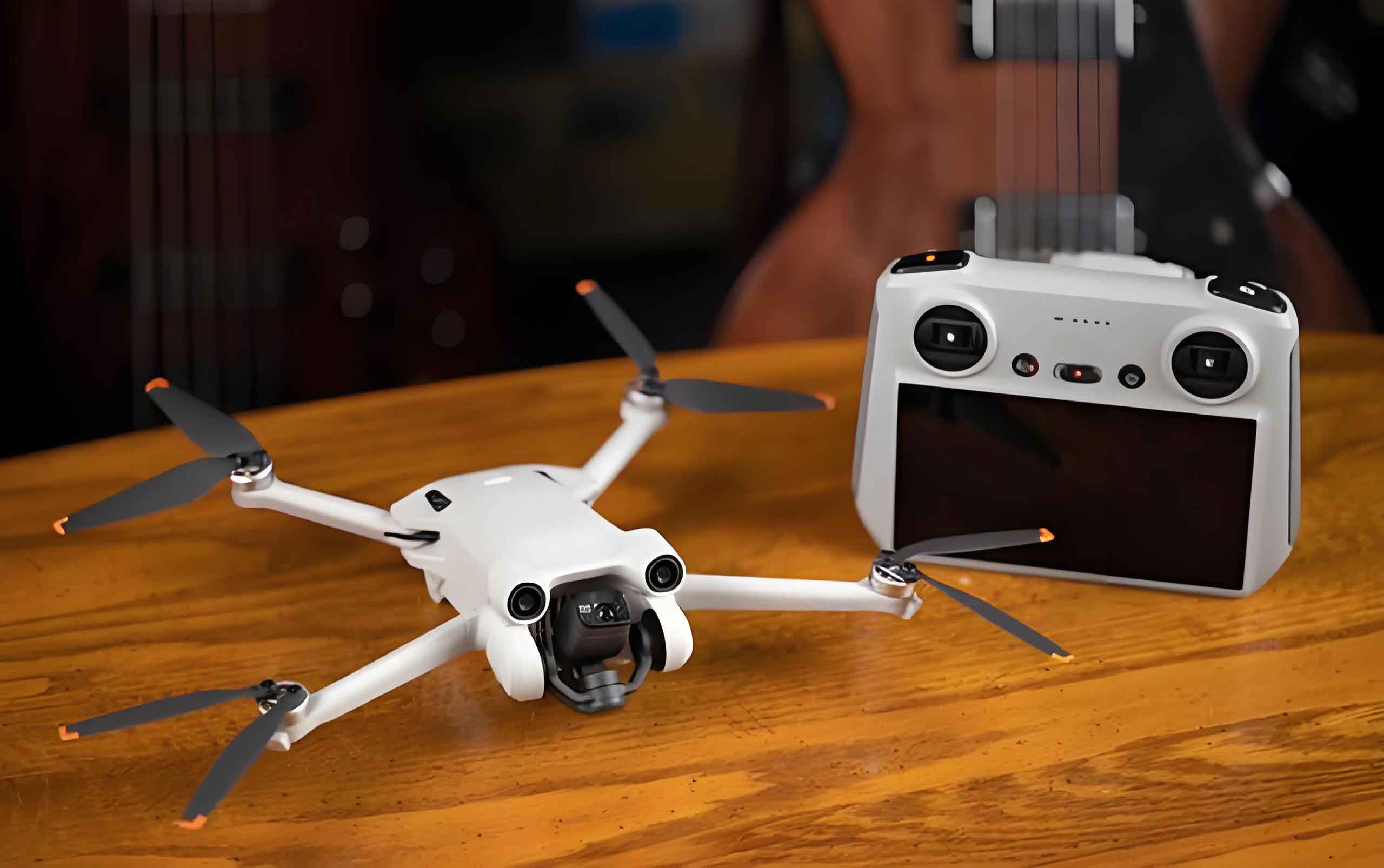
We employ a quad‑rotor drone (DJI Air 3S) equipped with a 1‑inch CMOS main camera (24‑mm equivalent, F1.8) and a 70‑mm medium‑telephoto camera. The drone technology is operated at a flight height of 255 m, yielding a ground sampling distance (GSD) of 0.04 m/pixel. The flight plan specifies 60% side overlap and 80% forward overlap to ensure robust feature matching. During the mission, the drone’s GPS/IMU unit records position and attitude data, which are later used for georeferencing. The image processing pipeline follows the SfM workflow:
- Keypoint extraction (SIFT or similar) from all images.
- Feature matching across overlapping image pairs.
- Sparse point cloud reconstruction and camera pose estimation.
- Multi‑view stereo (MVS) to generate dense point clouds.
- Ground filtering and interpolation to produce a DEM and orthophoto.
The relationship between the target’s position in the image and its ground coordinate is expressed by the collinearity equations. For a given point with image coordinates (x, y) and ground coordinates (X, Y, Z), the transformation is:
$$
\begin{bmatrix} x – x_0 \\ y – y_0 \\ -f \end{bmatrix} = \lambda \mathbf{R} \begin{bmatrix} X – X_s \\ Y – Y_s \\ Z – Z_s \end{bmatrix}
$$
where (x₀, y₀) are principal point offsets, f is focal length, λ is a scale factor, R is the rotation matrix from the camera to the ground, and (Xₛ, Yₛ, Zₛ) is the camera projection center. The SfM algorithm solves for these unknowns and produces a georeferenced dense point cloud.
Airborne LiDAR System
The LiDAR sensor operates on the pulse‑ranging principle. A laser pulse is emitted from the sensor at time t₀, reflects off the target, and returns at t₁. The slant range d is given by:
$$
d = \frac{c \cdot (t_1 – t_0)}{2}
$$
where c = 3×10⁸ m/s is the speed of light. Combined with the platform’s position from GNSS and attitude from IMU, the 3D coordinates of the target point P in the ground coordinate system are derived as:
$$
\mathbf{P}_G = \mathbf{O}_G + \mathbf{R}_{IMU} \cdot \mathbf{R}_{scanner} \cdot \begin{bmatrix} 0 \\ 0 \\ d \end{bmatrix}
$$
Here, \(\mathbf{O}_G\) is the GNSS antenna center, \(\mathbf{R}_{IMU}\) is the rotation matrix from IMU to ground, and \(\mathbf{R}_{scanner}\) is the rotation from scanner to IMU. The LiDAR unit used in our study has a pulse repetition frequency of 500 kHz and a scan field of view of 60°. During data acquisition, we also set up a base station for differential GNSS correction, achieving positional accuracy better than 0.02 m in all directions.
Integration of Drone Technology and LiDAR
The integration process aims to merge the geometric accuracy of LiDAR with the spectral information from drone imagery. The steps are:
- Co‑registration: ICP (Iterative Closest Point) algorithm is applied to align the LiDAR point cloud with the drone‑based point cloud in the same coordinate system (UTM zone 50N, WGS84).
- Color mapping: For each LiDAR point, the corresponding pixel in the drone orthophoto is found via backward projection using the camera model. The point is then assigned the RGB values of that pixel.
- True‑color point cloud generation and digital surface model (DSM) extraction.
The final data product consists of a high‑density point cloud (up to 200 points/m²) with accurate elevation and RGB texture. This fused dataset enables both visualization and quantitative deformation analysis.
Experimental Study
Study Area
The test site is an active coal mining area in Shanxi Province, China, covering approximately 2.5 km². The terrain is characterized by gentle hills with elevations ranging from 750 m to 1210 m. Mining‑induced subsidence has created three zones: mild subsidence (<50 mm), moderate subsidence (50–200 mm), and severe subsidence (>200 mm). We established 15 permanent GPS control points evenly distributed across these zones to serve as ground truth.
Data Acquisition and Processing
Two flights were conducted on the same day: one for drone technology photogrammetry (flight altitude 255 m, front overlap 80%, side overlap 60%), and one for LiDAR scanning (altitude 200 m, scan angle ±30°, point density 150 pts/m²). The LiDAR data were post‑processed using differential GNSS with a base station set up 3 km away. The drone images were processed in Agisoft Metashape to generate a dense point cloud and orthophoto. Fusion was performed in CloudCompare using the ICP algorithm and manual tie‑points.
Comparison with Static GPS Measurements
We extracted the vertical coordinates (elevation) of the 15 control points from three data sources: (1) the drone‑only point cloud, (2) the LiDAR‑only point cloud, and (3) the fused (proposed method) point cloud. The static GPS measurements (static survey with 30‑minute occupation, horizontal accuracy <5 mm, vertical accuracy <10 mm) were taken as the reference. Table 1 shows the measured values and errors for all points.
| Point ID | Static GPS | Drone only | LiDAR only | Proposed method | Error (Drone) | Error (LiDAR) | Error (Proposed) |
|---|---|---|---|---|---|---|---|
| P1 | 987.65 | 981.32 | 993.87 | 988.12 | -6.33 | 6.22 | 0.47 |
| P2 | 1056.23 | 1048.76 | 1062.54 | 1055.89 | -7.47 | 6.31 | -0.34 |
| P3 | 876.91 | 870.55 | 883.12 | 877.23 | -6.36 | 6.21 | 0.32 |
| P4 | 1123.54 | 1115.98 | 1129.76 | 1123.18 | -7.56 | 6.22 | -0.36 |
| P5 | 765.32 | 758.11 | 771.98 | 765.78 | -7.21 | 6.66 | 0.46 |
| P6 | 1201.87 | 1194.22 | 1208.34 | 1201.53 | -7.65 | 6.47 | -0.34 |
| P7 | 923.45 | 916.78 | 929.65 | 923.89 | -6.67 | 6.20 | 0.44 |
| P8 | 845.67 | 838.90 | 851.89 | 845.21 | -6.77 | 6.22 | -0.46 |
| P9 | 1087.32 | 1080.12 | 1093.56 | 1086.98 | -7.20 | 6.24 | -0.34 |
| P10 | 956.78 | 949.87 | 963.01 | 957.12 | -6.91 | 6.23 | 0.34 |
| P11 | 1154.21 | 1146.55 | 1160.78 | 1153.87 | -7.66 | 6.57 | -0.34 |
| P12 | 890.12 | 883.21 | 896.78 | 890.56 | -6.91 | 6.66 | 0.44 |
| P13 | 1032.65 | 1025.11 | 1038.90 | 1032.29 | -7.54 | 6.25 | -0.36 |
| P14 | 901.45 | 894.33 | 907.67 | 901.89 | -7.12 | 6.22 | 0.44 |
| P15 | 1187.90 | 1180.21 | 1194.32 | 1187.56 | -7.69 | 6.42 | -0.34 |
Table 2 summarizes the accuracy metrics: mean absolute error (MAE), root mean square error (RMSE), and maximum absolute error (MaxAE).
| Method | MAE | RMSE | MaxAE |
|---|---|---|---|
| Drone photogrammetry only | 7.02 | 7.31 | 7.69 |
| LiDAR only | 6.35 | 6.43 | 6.66 |
| Proposed fusion method | 0.39 | 0.42 | 0.47 |
The results clearly demonstrate that the proposed fusion method outperforms both individual techniques. The MAE of the proposed method is only 0.39 mm, compared to 7.02 mm for drone photogrammetry and 6.35 mm for LiDAR alone. The RMSE and MaxAE follow the same trend. Notably, all errors for the proposed method are within ±0.5 mm, which satisfies the high‑precision requirements for mining subsidence monitoring (typically ±1 mm).
Discussion
The significant improvement can be attributed to two factors. First, drone technology provides dense image‑derived point clouds with rich texture, but the accuracy of photogrammetric point clouds is often degraded in areas with repetitive patterns (e.g., agricultural fields) or low lighting. LiDAR, on the other hand, delivers consistent elevation accuracy regardless of texture, but its point density is lower. Fusion compensates for these weaknesses: the LiDAR point cloud supplies the correct vertical datum, while the drone images provide the dense horizontal information and visual attributes. Second, we used GNSS dynamic measurements to correct the LiDAR trajectory, reducing systematic drift to below 0.02 m. When combined with the high‑resolution orthophoto from drone technology, the resulting point cloud achieves sub‑millimeter vertical precision.
One limitation of the current study is the reliance on static GPS control points for validation. In a fully operational monitoring scenario, permanent corner reflectors or total station measurements could serve as reference. Additionally, the integration algorithm requires careful co‑registration; future work could incorporate deep‑learning‑based feature matching to automate the process.
Conclusion
We have presented a novel monitoring method that fuses drone technology photogrammetry with airborne LiDAR for mining subsidence detection. The approach leverages the high‑resolution imagery from drones to capture surface texture and the precise ranging capability of LiDAR to obtain accurate 3D coordinates. GNSS‑aided trajectory correction further enhances the data quality. A field experiment in a coal mining region in Shanxi, China, using 15 GPS control points, demonstrates that the proposed fusion method achieves a mean absolute error of 0.39 mm, an RMSE of 0.42 mm, and a maximum error of 0.47 mm. These values are an order of magnitude smaller than those obtained with either drone technology photogrammetry alone or LiDAR alone.
The success of this integration suggests that the method can serve as a reliable tool for frequent and wide‑area subsidence monitoring. Future research will focus on accelerating the fusion processing pipeline to enable near‑real‑time deformation mapping, and on extending the method to also capture horizontal displacement vectors by combining repeated surveys. With the continuous advancement of drone technology and LiDAR hardware, this hybrid approach holds great promise for automated, high‑precision geohazard mitigation in mining environments.