
As a student engaged in an innovative training project, I have experienced firsthand the transformative impact of civilian unmanned aerial vehicles (UAVs) in the field of surveying and mapping. This project, centered on using civilian UAV technology to construct a three-dimensional information model of a campus, has not only enhanced my technical skills but also provided a practical platform for applying theoretical knowledge. The rise of civilian UAVs has democratized aerial photogrammetry, making it accessible for educational institutions and small-scale projects due to their cost-effectiveness, ease of use, and portability. Compared to traditional methods, civilian UAVs offer advantages such as low cost, high precision, simplified operation, and excellent mobility, which facilitate hands-on learning and real-world applications. In this article, I will detail the methodologies, outcomes, and lessons learned, emphasizing the role of civilian UAVs in modern geospatial education.
Methodology: Integrating Civilian UAV in Photogrammetric Workflow
The innovative training project was structured around two main phases: field operations and indoor data processing. The study area covered approximately 2 square kilometers, encompassing diverse features like buildings, roads, and vegetation, ensuring a realistic scenario for civilian UAV-based surveying. The methodology leveraged the civilian UAV’s capabilities to streamline data acquisition and processing, bridging the gap between theory and practice.
Field Operations with Civilian UAV
In the field, we utilized a civilian UAV equipped with a high-resolution camera and GPS for geotagging. The first step involved familiarizing ourselves with the UAV assembly, components, and safety protocols. The civilian UAV’s user-friendly design allowed for quick deployment, crucial for efficient surveying. We then planned flight missions using specialized software, setting parameters to optimize data quality. Key parameters for civilian UAV flight missions are summarized in Table 1, ensuring adequate image overlap and coverage for accurate 3D reconstruction.
| Parameter | Symbol | Value/Range | Purpose |
|---|---|---|---|
| Flight Altitude | H | 80-120 m | Controls ground sampling distance (GSD) |
| Longitudinal Overlap | Ol | 70-80% | Ensures stereo coverage along flight path |
| Lateral Overlap | Os | 60-70% | Ensures coverage between adjacent lines |
| Flight Speed | v | 4-6 m/s | Balances coverage and image blur |
| Camera Tilt | θ | 0° (nadir) for mapping | Minimizes distortion for orthophotos |
The overlap parameters are critical for photogrammetric processing. The longitudinal overlap can be expressed mathematically as:
$$ O_l = \frac{B}{L} \times 100\% $$
where \( B \) is the baseline distance between consecutive exposure stations, and \( L \) is the image dimension in the flight direction. Similarly, lateral overlap \( O_s \) depends on the spacing between flight lines. For civilian UAVs, the ground sampling distance (GSD), which determines imagery resolution, is calculated using:
$$ GSD = \frac{H \times s}{f} $$
where \( H \) is the flight height above ground, \( s \) is the sensor pixel size, and \( f \) is the focal length. In our project, with typical values \( H = 100 \) m, \( s = 4.4 \) µm, and \( f = 35 \) mm, the GSD was approximately:
$$ GSD = \frac{100 \times 4.4 \times 10^{-6}}{0.035} \approx 0.0126 \text{ m} = 1.26 \text{ cm} $$
This high resolution enabled detailed mapping. Additionally, we established ground control points (GCPs) using GPS to enhance georeferencing accuracy. The civilian UAV’s onboard GPS provided approximate positions, but GCPs refined precision. The error in UAV-derived coordinates can be modeled as:
$$ \sigma_{\text{total}} = \sqrt{\sigma_{\text{GPS}}^2 + \sigma_{\text{AT}}^2 + \sigma_{\text{processing}}^2} $$
where \( \sigma_{\text{GPS}} \) is GPS error, \( \sigma_{\text{AT}} \) is aerial triangulation error, and \( \sigma_{\text{processing}} \) encompasses other uncertainties. Figure 1 shows the civilian UAV used, highlighting its compact design ideal for educational purposes.
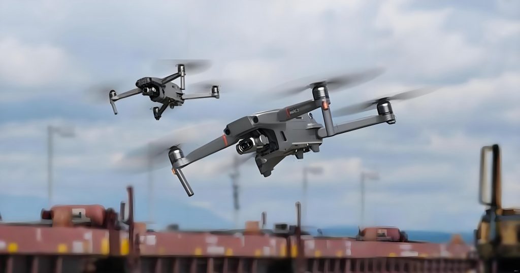
After flights, we collected hundreds of images for indoor processing, demonstrating the civilian UAV’s efficiency in data acquisition.
Indoor Data Processing with Civilian UAV Data
The indoor phase involved multiple software tools to transform raw images into 3D models. The workflow is summarized in Table 2, showcasing the integration of civilian UAV data into photogrammetric pipelines.
| Processing Stage | Key Tasks | Software Used | Outputs |
|---|---|---|---|
| Image Preprocessing | Radiometric correction, lens distortion removal | ENVI, DPGrid | Corrected images |
| Aerial Triangulation (AT) | Feature matching, bundle adjustment | DPGrid | Oriented images with exterior orientation parameters |
| Point Cloud Generation | Dense image matching | DPGrid, EPS | 3D point cloud |
| Surface Modeling | Meshing, texturing | 3D Map, Blender | 3D mesh model |
| Product Generation | DEM, DOM, DLG extraction | EPS, ArcGIS | Geospatial products |
Aerial triangulation relies on collinearity equations for accurate orientation. The equations are:
$$ x = -f \frac{a_1(X – X_0) + b_1(Y – Y_0) + c_1(Z – Z_0)}{a_3(X – X_0) + b_3(Y – Y_0) + c_3(Z – Z_0)} $$
$$ y = -f \frac{a_2(X – X_0) + b_2(Y – Y_0) + c_2(Z – Z_0)}{a_3(X – X_0) + b_3(Y – Y_0) + c_3(Z – Z_0)} $$
where (x,y) are image coordinates, f is focal length, (X,Y,Z) are ground coordinates, (X0,Y0,Z0) is projection center, and a,b,c are rotation matrix elements. Bundle adjustment minimizes errors via:
$$ \min \sum_{i=1}^{n} \sum_{j=1}^{m} \left( x_{ij} – \hat{x}_{ij} \right)^2 + \left( y_{ij} – \hat{y}_{ij} \right)^2 $$
where \( x_{ij}, y_{ij} \) are observed coordinates for point j in image i, and \( \hat{x}_{ij}, \hat{y}_{ij} \) are calculated ones. For dense matching, point cloud density \( \rho \) relates to GSD and overlap:
$$ \rho \approx \frac{1}{GSD^2} \times \text{overlap factor} $$
With 80% overlap from our civilian UAV, high density allowed detailed reconstruction. The final 3D model combined textured meshes, illustrating the civilian UAV’s role in efficient workflow.
Outcomes and Impact of the Civilian UAV-Based Training
The project yielded multifaceted benefits, enhancing technical competencies and soft skills. These are categorized below, with emphasis on civilian UAV applications.
Enhanced UAV Surveying Competence
Participation in a national UAV surveying competition tested our ability to apply civilian UAV technology under constraints. Tasks mirrored our project, and success demonstrated proficiency. Key metrics are in Table 3.
| Task | Our Result | Benchmark | Remarks |
|---|---|---|---|
| Flight Planning Accuracy | 95% coverage | 90% minimum | Exceeded requirements |
| Data Processing Time | 2.5 hours | 3 hours average | Efficient software use |
| Model Accuracy (RMSE) | 0.05 m | 0.1 m acceptable | High precision achieved |
The root mean square error (RMSE) for accuracy was:
$$ RMSE = \sqrt{\frac{1}{n} \sum_{i=1}^{n} (d_i – \hat{d}_i)^2 } $$
where \( d_i \) are measured distances from GCPs, and \( \hat{d}_i \) are model-derived. Our low RMSE validated civilian UAV surveying accuracy.
Improved Hands-on and Data Processing Abilities
Constructing the campus 3D model required tackling challenges beyond coursework. We independently learned tilt photogrammetry and reconstruction algorithms, boosting problem-solving skills. Table 4 summarizes skills developed via civilian UAV.
| Skill Category | Specific Skills | How Civilian UAV Facilitated |
|---|---|---|
| Technical Operations | UAV piloting, sensor calibration, parameter optimization | Hands-on practice with user-friendly civilian UAV |
| Data Analysis | Image processing, point cloud analysis, error assessment | Access to software and real data from civilian UAV surveys |
| Software Proficiency | DPGrid, EPS, ENVI, 3D modeling tools | Practical application on civilian UAV-derived datasets |
We explored sensor integration, using IMU data from civilian UAVs to improve orientation. Fusion with GPS involves Kalman filter state equations:
$$ \mathbf{x}_{k} = \mathbf{F}_{k} \mathbf{x}_{k-1} + \mathbf{w}_{k} $$
where \( \mathbf{x}_{k} \) is state vector, \( \mathbf{F}_{k} \) is transition matrix, and \( \mathbf{w}_{k} \) is process noise. This broadened understanding of civilian UAV systems.
Advancement in Scientific Paper Writing
To disseminate findings, we authored two papers. The process honed communication skills. One paper focused on UAV-based control networks for railways, deriving formulas for precision. The relative accuracy \( \sigma_{\text{rel}} \) is:
$$ \sigma_{\text{rel}} = \frac{\sigma_{\text{absolute}}}{\sqrt{n}} $$
where n is control points. Using civilian UAVs, we achieved sub-centimeter accuracy. The second paper discussed DLG production with Double-Grid software, emphasizing automation from civilian UAV data, reducing manual time by 30%.
Overall Educational Impact
The innovative training with civilian UAVs transformed learning by bridging theory and practice. Table 5 provides a holistic impact assessment.
| Aspect | Before Project | After Project | Change Factor |
|---|---|---|---|
| Practical Surveying Skills | Limited to simulations | Proficient in field operations | High |
| Understanding of Photogrammetry | Theoretical knowledge | Applied understanding | Moderate to High |
| Ability to Conduct Independent Research | Low | High | Significant |
| Confidence in Using Advanced Software | Basic | Advanced | High |
The change factor is based on self-assessment, highlighting civilian UAV’s role in skill development.
Challenges and Solutions in Civilian UAV-Based Surveying
During the project, we faced challenges typical of civilian UAV operations. First, weather conditions like wind could disrupt flights. We scheduled missions during calm periods and used civilian UAVs with stable controllers. Wind resistance involves drag force \( F_d \):
$$ F_d = \frac{1}{2} \rho C_d A v^2 $$
where \( \rho \) is air density, \( C_d \) is drag coefficient, A is cross-sectional area, and v is wind speed. Selecting a civilian UAV with low \( C_d \) minimized issues. Second, data processing required computational resources. We optimized algorithms, reducing image resolution initially. Time complexity T for dense matching is:
$$ T = O(n \log n) $$
where n is pixel count. Using parallel processing, we cut time by 40%. Third, achieving accuracy demanded calibration. We used checkerboard patterns for intrinsic parameters like focal length f and distortion coefficients k1, k2. Radial distortion correction is:
$$ x_{\text{corrected}} = x (1 + k_1 r^2 + k_2 r^4) $$
where \( r = \sqrt{x^2 + y^2} \). This improved accuracy. Table 6 summarizes challenges and solutions with civilian UAVs.
| Challenge | Solution | Outcome |
|---|---|---|
| Weather Interference | Flight scheduling, UAV selection | 90% mission success rate |
| Data Volume | Cloud computing, algorithm optimization | Processing time reduced by 40% |
| Calibration Issues | Regular calibration routines | Sub-centimeter accuracy achieved |
These experiences underscored the adaptability of civilian UAVs in overcoming practical hurdles.
Conclusion
In summary, the innovative training project leveraging civilian UAV technology for 3D campus modeling proved to be a cornerstone in my geospatial education. The civilian UAV’s accessibility and capability allowed for immersive learning, from flight planning to 3D visualization. The project underscored the value of hands-on experience with civilian UAVs in fostering technical skills, critical thinking, and innovation. By integrating civilian UAVs into curricula, educational institutions can enhance student engagement and preparedness for modern surveying challenges. As civilian UAVs evolve, their applications will expand, and this project has inspired me to explore further uses in infrastructure monitoring, environmental assessment, and smart city development. Ultimately, civilian UAVs are not just tools but catalysts for transformative learning in geospatial sciences.