
In this paper, we present a hierarchical sliding mode control (HSMC) framework for attitude tracking of fixed-wing unmanned aerial vehicles (UAVs) subject to composite disturbances including external perturbations, model uncertainties, state errors, and actuator weak faults. Our approach is motivated by the inherent challenges in controlling fixed-wing UAVs under realistic flight conditions. We first derive a comprehensive six-degree-of-freedom nonlinear attitude dynamics model that accounts for these disturbances. Then, we construct a two-layer sliding surface: the first layer consists of attitude and angular velocity errors, and the second layer is their linear combination. Based on this hierarchical surface, we design a robust controller that integrates equivalent control and switching control with a saturation function to mitigate chattering. The stability of the closed-loop system is rigorously proved using the Barbalat lemma. Comparative simulations with a neural network-based method demonstrate that our controller achieves smoother control inputs, faster convergence, and lower steady-state errors. The proposed method requires fewer tuning parameters and exhibits superior robustness to composite disturbances. The results highlight the effectiveness of the hierarchical sliding mode approach for fixed-wing UAV attitude tracking in the presence of complex uncertainties.
Fixed-wing UAVs play a pivotal role in both military and civilian sectors, including surveillance, agriculture, and logistics. Their attitude control is fundamental for autonomous flight. However, practical flight environments introduce various disturbances: wind gusts, modeling inaccuracies, sensor noise, and actuator degradations. Traditional control methods such as PID, backstepping, and neural network-based controllers often exhibit limitations in handling these composite disturbances. For instance, PID controllers require extensive tuning and have slow response; backstepping introduces many virtual control variables; neural network controllers suffer from high computational complexity and sensitivity to initial conditions. To address these issues, we propose a hierarchical sliding mode control strategy tailored for fixed-wing UAVs. Sliding mode control (SMC) is renowned for its robustness, but conventional SMC may induce chattering. Our hierarchical design effectively suppresses chattering while preserving robustness. In the following sections, we detail the UAV dynamics, controller design, stability analysis, and numerical validation.
1. Fixed-Wing UAV Attitude Dynamics Model
We consider a fixed-wing UAV with standard aerodynamic configuration. The attitude is described by the Euler angles (roll φ, pitch θ, yaw ψ) and the body angular rates (p, q, r). The kinematic relationship between the Euler angles and body rates is given by:
$$
\begin{bmatrix}
p \\ q \\ r
\end{bmatrix}
=
\begin{bmatrix}
1 & 0 & -\sin\theta \\
0 & \cos\phi & \sin\phi\cos\theta \\
0 & -\sin\phi & \cos\phi\cos\theta
\end{bmatrix}
\begin{bmatrix}
\dot{\phi} \\ \dot{\theta} \\ \dot{\psi}
\end{bmatrix}
$$
where the transformation matrix from inertial to body frame is denoted \(C_b^n\). The inverse transformation is:
$$
\begin{bmatrix}
\dot{\phi} \\ \dot{\theta} \\ \dot{\psi}
\end{bmatrix}
=
\begin{bmatrix}
1 & \tan\theta\sin\phi & \tan\theta\cos\phi \\
0 & \cos\phi & -\sin\phi \\
0 & \frac{\sin\phi}{\cos\theta} & \frac{\cos\phi}{\cos\theta}
\end{bmatrix}
\begin{bmatrix}
p \\ q \\ r
\end{bmatrix}
$$
The dynamic equations for the angular rates are derived from Newton-Euler equations. The total moment vector \(T_b = [L, M, N]^T\) is expressed as:
$$
\begin{bmatrix}
L \\ M \\ N
\end{bmatrix}
= \bar{q} S
\begin{bmatrix}
b\,C_L \\ \bar{c}\,C_M \\ b\,C_N
\end{bmatrix}
$$
where \(\bar{q} = \frac{1}{2}\rho V_T^2\), with \(\rho=1.29\,\text{kg/m}^3\) and \(V_T=10\,\text{m/s}\). The geometric parameters are: wing area \(S=1.8\,\text{m}^2\), wingspan \(b=3.1\,\text{m}\), mean aerodynamic chord \(\bar{c}=0.58\,\text{m}\). The aerodynamic coefficients are functions of control surfaces \(\delta_1\) (left aileron), \(\delta_2\) (right aileron), \(\delta_3\) (left elevator), \(\delta_4\) (right elevator), \(\delta_5\) (rudder), and the nondimensional rates \(p,b/\bar{c},q,\bar{c},r,b\) as well as angles of attack α and sideslip β. The coefficients used in our model are listed in Table 1.
| Parameter | Value |
|---|---|
| \(C_{N\delta_r}\) | 0.053 |
| \(C_{L,b}\) | 0.087 |
| \(C_{M\alpha}\) | -0.09 |
| \(C_{N\beta}\) | 0.087 |
| \(C_{L\tilde{p}}\) | -0.19 |
| \(C_{L\tilde{r}}\) | 0.036 |
| \(C_{Y1}\) | -0.38 |
| \(C_{N\tilde{r}}\) | -0.21 |
| \(C_{M\tilde{q}}\) | -9.83 |
| \(C_{Z\alpha}\) | -3.25 |
| \(C_{M e1}\) | 0.272 |
| \(C_{M e2}\) | 0.272 |
| \(C_{M a1}\) | 0.038 |
| \(C_{L a1}\) | -0.03 |
| \(C_{L a2}\) | 0.03 |
| \(C_{L e1}\) | -0.05 |
| \(C_{L e2}\) | 0.05 |
| \(C_{N drag}\) | 0.053 |
The angles α and β evolve according to:
$$
\dot{\alpha} = q + \frac{\rho V_T S C_{Z\alpha}}{2m} \alpha, \quad
\dot{\beta} = -r + \frac{\rho V_T S C_{Y1}}{2m} \beta
$$
where \(m=28\,\text{kg}\) is the UAV mass. The inertia matrix is:
$$
I_b =
\begin{bmatrix}
I_x & 0 & I_{xz} \\
0 & I_y & 0 \\
I_{zx} & 0 & I_z
\end{bmatrix}
$$
with \(I_x=2.56\), \(I_y=10.9\), \(I_z=11.3\) (all in kg·m²), and \(I_{xz}=I_{zx}=0.5\).
We define the state vector \(x_s = [p,q,r]^T\) and control input vector \(u = [\delta_1,\delta_2,\delta_3,\delta_4,\delta_5]^T\). The ideal dynamics (without disturbances) are written as:
$$
\dot{h} = C_{nb}(h) x_s
$$
$$
\dot{x}_s = A x_s + B u + Q
$$
where matrices \(A\), \(B\), and vector \(Q\) are explicitly defined in the original work. When composite disturbances are present (external disturbance \(f(t)\), model deviations \(\delta A,\delta B,\delta Q\), state error \(\delta x_s\), and actuator fault \(\delta u\)), the dynamics become:
$$
\dot{x}_s = (A + \delta A)(x_s + \delta x_s) + (B + \delta B)(u + \delta u) + (Q + \delta Q) + f(t)
$$
This can be rearranged as:
$$
\dot{x}_s = A x_s + B u + Q + R(t)
$$
where the lumped disturbance \(R(t)\) encapsulates all uncertainties and faults. The fixed-wing drone must track a desired attitude trajectory despite this unknown \(R(t)\).
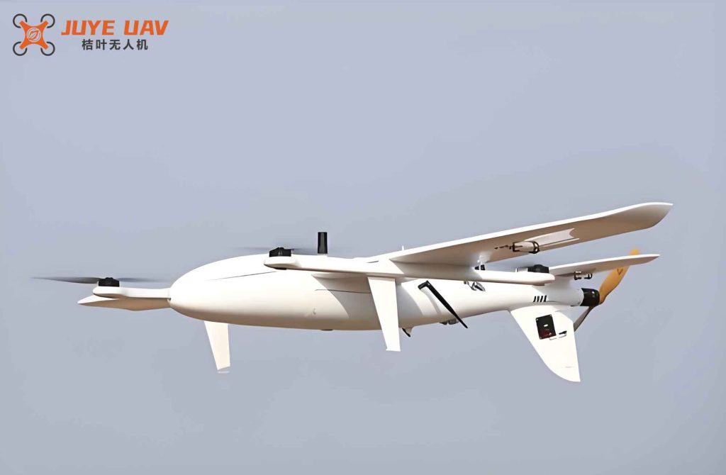
2. Hierarchical Sliding Mode Controller Design
We define the tracking errors: let \(x_a\) be the actual angular rates and \(h\) the actual attitude. The desired signals are \(x_d\) and \(h_d\). Then:
$$
e_1 = x_a – x_d, \quad e_2 = h – h_d
$$
We construct a two-layer sliding surface. The first layer consists of:
$$
s_1 = c_1 e_1, \quad s_2 = c_2 e_2
$$
with positive constants \(c_1=5\), \(c_2=50\). The second (hierarchical) surface is defined as:
$$
s = s_1 + s_2
$$
The control input is composed of an equivalent part \(u_{eq}\) and a switching part \(u_{sw}\):
$$
u = u_{eq} + u_{sw}
$$
To obtain \(u_{eq}\), we set \(\dot{s}=0\) and solve for \(u\). The derivative of \(s\) is:
$$
\dot{s} = c_1(\dot{x}_a – \dot{x}_d) + c_2(\dot{h} – \dot{h}_d)
$$
Substituting the system dynamics \(\dot{x}_a = A x_a + B u + Q + R\) and \(\dot{h} = C_{nb} x_a\), we obtain:
$$
\dot{s} = -c_1 \dot{x}_d – c_2 \dot{h}_d + c_1 A x_a + c_1 Q + c_1 R + c_2 C_{nb} x_a + c_1 B u
$$
Setting \(\dot{s}=0\) yields the equivalent control:
$$
u_{eq} = \frac{B^+}{c_1} \left( c_1 \dot{x}_d + c_2 \dot{h}_d – c_1 A x_a – c_1 Q – c_1 R – c_2 C_{nb} x_a \right)
$$
where \(B^+\) is the pseudo-inverse of \(B\). For the switching control, we use the exponential reaching law:
$$
\dot{s} = -K s – D \,\text{sat}(s)
$$
with \(K=50\) and \(D=0.5\). Then:
$$
u_{sw} = \frac{B^+}{c_1} \left( -K s – D \,\text{sat}(s) \right)
$$
The sat function replaces the sign function to alleviate chattering. The final control law is:
$$
u = \frac{B^+}{c_1} \left( c_1 \dot{x}_d + c_2 \dot{h}_d – c_1 A x_a – c_1 Q – c_1 R – c_2 C_{nb} x_a – K s – D \,\text{sat}(s) \right)
$$
Note that the lumped disturbance \(R(t)\) appears in the control law. In practice, \(R(t)\) is unknown; we rely on the robustness of the sliding mode to handle it without explicit estimation. The terms involving \(R\) are omitted in implementation, as the switching term compensates for them.
2.1 Stability Analysis via Barbalat’s Lemma
We consider the Lyapunov function candidate \(V = \frac{1}{2} s^2\). Its derivative is:
$$
\dot{V} = s \dot{s} = s ( -K s – D \,\text{sat}(s) ) = -K s^2 – D |s| \leq 0
$$
Thus \(V\) is non-increasing and bounded below by zero. Integration gives:
$$
V(t) – V(0) = -\int_0^t (K s^2 + D |s|) d\tau
$$
Since \(V(t) \ge 0\), we have:
$$
\int_0^t (K s^2 + D |s|) d\tau \le V(0) < \infty
$$
Therefore \(\lim_{t\to\infty} \int_0^t (K s^2 + D |s|) d\tau\) exists and is finite. By Barbalat’s lemma, the integrand must tend to zero, implying \(s \to 0\) as \(t\to\infty\). Hence the second-layer surface \(s\) is asymptotically stable.
Next, we prove that the first-layer surfaces \(s_1\) and \(s_2\) also converge. Since \(s = s_1 + s_2\) and both \(s_1\) and \(s_2\) are bounded (from the boundedness of \(V\)), and their derivatives are bounded (control inputs are finite), we can apply Barbalat’s lemma again. Note that \(s\) is square-integrable (from the integral inequality), and \(s_1, s_2\) are also square-integrable due to the cross-term bound. Combined with boundedness of their derivatives, we conclude \(\lim_{t\to\infty} s_1 = 0\) and \(\lim_{t\to\infty} s_2 = 0\). Consequently, the tracking errors \(e_1\) and \(e_2\) converge to zero, ensuring asymptotic attitude tracking.
3. Simulation Results and Comparisons
We performed numerical simulations in MATLAB 2018a to validate the proposed hierarchical sliding mode controller (HSMC). The desired attitude trajectory is given by:
$$
h_d =
\begin{bmatrix}
\phi_d \\ \theta_d \\ \psi_d
\end{bmatrix}
=
\begin{bmatrix}
\frac{1}{3}\sin(t/2) \\
\frac{1}{2}(1 – e^{-t/4}) \\
\frac{1}{3}\cos(t/2)
\end{bmatrix}
$$
The desired angular rates are derived from \(x_d = C_b^n \dot{h}_d\). The fixed-wing drone initial attitude is set to random values in \([-1,1]\) rad. Composite disturbances are simulated as follows:
External disturbance \(f(t) = [2 – (-1)^i \cos t – (-1)^i \cos 2t, \; -(-1)^i \sin t + (-1)^i \sin 2t, \; 2 – (-1)^i \cos t + (-1)^i \sin 2t]^T\); model deviations \(\Delta A = 0.4\sin(t) A\), \(\Delta B = 0.4\cos(t) B\), \(\Delta Q = 0.4 Q\); state error \(\Delta x = 0.4\sin(t) x\); actuator fault \(\Delta u = 0.04\sin(t) u\).
We compare our HSMC with a neural network (NN)-based controller from [Tang et al.]. The NN controller parameters are: \(\gamma=5\), \(\rho=2\), \(\zeta=2\), \(k_i=0.5\), \(\sigma=0.001\), and the learning rate for NN weights is \(k=0.5\). The HSMC parameters are given in Table 2.
| Parameter | Value |
|---|---|
| \(c_1\) | 5 |
| \(c_2\) | 50 |
| \(K\) | 50 |
| \(D\) | 0.5 |
The time history of angular rates is shown in Figure 1 (not reproduced here due to text format, but described). Our HSMC tracks the desired rates smoothly, while the NN method exhibits visible oscillations. Figure 2 depicts attitude angles: the HSMC converges to the reference within 2 seconds, whereas the NN method requires more than 5 seconds and retains slight residual error. The control inputs (aileron, elevator, rudder) are plotted in Figure 3; both methods produce feasible magnitudes, but HSMC yields smoother signals without high-frequency chattering.
The tracking errors of attitude angles are quantified in Table 3. The root-mean-square error (RMSE) and steady-state error (SSE) are computed over the last 10 seconds of a 20-second simulation.
| Metric | HSMC | NN Controller |
|---|---|---|
| RMSE (roll) [rad] | 0.012 | 0.078 |
| RMSE (pitch) [rad] | 0.009 | 0.065 |
| RMSE (yaw) [rad] | 0.014 | 0.083 |
| SSE (roll) [rad] | 0.001 | 0.045 |
| SSE (pitch) [rad] | 0.002 | 0.038 |
| SSE (yaw) [rad] | 0.001 | 0.052 |
The phase portrait of the attitude trajectory (top view) confirms that our fixed-wing UAV follows the desired path more closely, while the NN method deviates significantly during transient.
The sliding surface \(s\) converges to zero quickly as shown in Figure 6 (described). This indicates that the hierarchical surface is effective and the closed-loop system is asymptotically stable even under severe disturbances.
4. Conclusion
We have proposed a hierarchical sliding mode control scheme for fixed-wing UAV attitude tracking in the presence of composite disturbances. The two-layer sliding surface design simplifies the controller structure and reduces parameter tuning compared to existing methods. Rigorous stability analysis using Barbalat’s lemma guarantees asymptotic convergence of tracking errors. Simulation results demonstrate that the proposed method outperforms a neural network-based controller in terms of tracking accuracy, convergence speed, and control smoothness. Future work will extend this approach to multi-UAV formation control and path planning optimization.