
As a researcher in autonomous systems, I have extensively explored the application of drone formations in various domains, from search and rescue to entertainment spectacles. In recent years, formation drone light shows have emerged as a captivating display of coordinated aerial robotics, where multiple drones synchronize their movements to create dynamic patterns and visual effects in the sky. However, orchestrating such formations in unknown or dynamic environments poses significant challenges, including real-time adaptation, collision avoidance, and efficient coverage. Traditional algorithms for drone swarm control often suffer from high computational loads and fail to fully leverage the distributed, cooperative nature of the group. To address these issues, I propose integrating a bio-inspired neural network (BINN) model with model predictive control (MPC) to enhance the performance and adaptability of formation drone light shows. This approach not only improves search capabilities in unknown areas but also ensures seamless and visually stunning light displays by enabling drones to interact rapidly with their environment and each other.
The core of my method lies in representing environmental state information through a BINN-based search model, which mimics the self-organizing behaviors observed in insect colonies. During a formation drone light show, this model utilizes excitation and inhibition functions to allow drones to quickly interact with the environment and the swarm, creating a comprehensive map of the area. Meanwhile, MPC guides the cluster formation, enhancing the ability to navigate and cover unknown regions while maintaining artistic precision. In this article, I will detail the design of the drone formation control method, the BINN-based environmental model, and provide simulation results that demonstrate the efficacy of this approach for formation drone light shows. By incorporating these advanced techniques, we can achieve higher coverage, better adaptability, and more efficient coordination, making formation drone light shows not only visually appealing but also robust and intelligent.
To begin, let me outline the drone dynamics model that forms the foundation of our control system. Each drone in the formation is assumed to be equipped with an autopilot for airspeed, heading, and flight path, incorporating three translational and two rotational degrees of freedom. This leads to an equivalent second-order system dynamics model, as shown in Equation (1).
$$
\begin{aligned}
\dot{x}_U &= V_U \cos \chi_U \cos \gamma_U \\
\dot{y}_U &= V_U \sin \chi_U \cos \gamma_U \\
\dot{z}_U &= V_U \sin \gamma_U \\
\dot{V}_U &= \frac{1}{\tau_v}(V_U^c – V_U) \\
\dot{\chi}_U &= \frac{1}{\tau_\chi}(\chi_U^c – \chi_U) \\
\dot{\gamma}_U &= \frac{1}{\tau_\gamma}(\gamma_U^c – \gamma_U)
\end{aligned}
$$
In these equations, $x_U$, $y_U$, and $z_U$ represent the drone’s velocity components along the x, y, and z axes, respectively. $V_U$ is the horizontal speed, $\chi_U$ is the heading angle, and $\gamma_U$ is the flight path angle. The derivatives $\dot{V}_U$, $\dot{\chi}_U$, and $\dot{\gamma}_U$ denote the rates of change, with control inputs $V_U^c$, $\chi_U^c$, and $\gamma_U^c$. The time constants $\tau_v$, $\tau_\chi$, and $\tau_\gamma$ characterize the system’s response. Additionally, practical constraints must be considered to ensure safe and feasible operations during a formation drone light show, as given in Equation (2).
$$
\begin{aligned}
V_{\text{min}} &\leq V_U \leq V_{\text{max}} \\
|\dot{\chi}_U| &\leq \frac{n_{\text{max}} g}{V_U} \\
\gamma_{\text{min}} &\leq \gamma_U \leq \gamma_{\text{max}}
\end{aligned}
$$
Here, $V_{\text{min}}$ and $V_{\text{max}}$ are the minimum and maximum horizontal speeds, $n_{\text{max}}$ is the maximum lateral load factor, $g$ is gravitational acceleration, and $\gamma_{\text{min}}$ and $\gamma_{\text{max}}$ are the limits for the flight path angle. These constraints are crucial for maintaining stability and safety in dense formations typical of formation drone light shows.
Next, I design the formation control using MPC. The position error $e_c$ and velocity error $e_v$ for the swarm are defined as follows:
$$
e_c = c_p – c_d, \quad e_v = \dot{c}_p – \dot{c}_d
$$
where $c_p$ is the current position, $c_d$ is the desired position, $\dot{c}_p$ is the current velocity, and $\dot{c}_d$ is the desired velocity. From this, a discrete state-space equation for the error dynamics is derived, as shown in Equation (5).
$$
\begin{bmatrix} e_U(k+1) \\ \dot{e}_U(k+1) \end{bmatrix} = \begin{bmatrix} 1 & \Delta t \\ 0 & 1 \end{bmatrix} \begin{bmatrix} e_U(k) \\ \dot{e}_U(k) \end{bmatrix} + \begin{bmatrix} \Delta t \\ 1 \end{bmatrix} u(k)
$$
In this equation, $e_U(k)$ and $\dot{e}_U(k)$ are the position and velocity errors at time step $k$, $\Delta t$ is the sampling time, and $u(k)$ is the input vector. This can be expressed in standard state-space form, as in Equation (6).
$$
x(k+1) = A x(k) + B u(k), \quad y(k+1) = C x(k+1)
$$
Here, $x(k)$ is the system state variable, $A$ and $B$ are coefficient matrices, $y(k)$ is the output variable, and $C$ is the output matrix. Since the error is used as the state variable, the output $y$ equals $x$. For MPC, I employ a quadratic programming (QP) approach to minimize a cost function, as formulated in Equation (7).
$$
q(z) = z^T H z + f^T z
$$
In this context, $q(z)$ is the optimization function, $z$ is the optimization variable, $H$ is a positive definite symmetric matrix weighting state tracking errors, and $f$ is a matrix related to reference trajectory deviations. The overall cost function $J$ is then given by Equation (8).
$$
J = J_q + J_r + J_f = \sum_{i=0}^{N-1} x(k+i|k)^T Q x(k+i|k) + \sum_{i=0}^{N-1} u(k+i|k)^T R u(k+i|k) + x(k+N|k)^T F x(k+N|k)
$$
Here, $J_q$ represents the weighted sum of errors, $J_r$ is the weighted system input, $J_f$ is the terminal error at the end of the prediction horizon, $N$ is the prediction horizon, $Q$, $R$, and $F$ are weighting matrices. By solving this QP problem to minimize $J$, we achieve effective cluster control for the formation drone light show, ensuring synchronized movements and obstacle avoidance.
To model the environment for the formation drone light show, I adopt a BINN-based approach. This model grids the task area into cells, each representing a neuron with an activity value. Inspired by collective biological behaviors, the BINN allows drones to interact through excitation and inhibition within a communication range $L_{\text{max}}$, facilitating dynamic environment mapping without global optimization. The neural activity is governed by Equation (9).
$$
\frac{dx_{j1}}{dt} = -A x_{j1} + (B – x_{j1}) \left([I_{j1}^e]^+ + \sum_{i=1}^{n} w_{j1,j2} x_{j2}\right) – (D + x_{j1}) [I_{j1}^o]^-
$$
In this equation, $x_{j1}$ is the activity of neuron $j1$, $A$ is the decay rate, $x_{j2}$ are activities of neighboring neurons, $B$ and $D$ are bounds on neuron activity, $I_{j1}^e$ and $I_{j1}^o$ are excitatory and inhibitory inputs, and $w_{j1,j2}$ are lateral connection weights computed as per Equation (10).
$$
w_{j1,j2} =
\begin{cases}
\frac{a}{\|p_{j1} – p_{j2}\|}, & \text{if } \|p_{j1} – p_{j2}\| \leq R_n \\
0, & \text{if } \|p_{j1} – p_{j2}\| > R_n
\end{cases}
$$
Here, $p_{j1}$ and $p_{j2}$ are position vectors of the neurons, $R_n$ is a distance threshold, and $a$ is a constant. Each grid cell in the map has three states: unsearched, searched, or obstacle, indicated by a state flag $I_i$ as in Equation (11).
$$
I_i =
\begin{cases}
1, & \text{if } S(G_i) = 1 \text{ (unsearched)} \\
0, & \text{if } S(G_i) = 0 \text{ (searched)} \\
-1, & \text{if } S(G_i) = -1 \text{ (obstacle)}
\end{cases}
$$
For target probability modeling in a formation drone light show, we consider the probability $p_{a,b}$ of a target existing at grid $(a,b)$. The target probability map (TPM) for drone $U$ at time $k$ is given by Equation (12).
$$
\text{TPM}_U(k) = \{ p_{a,b}(k) \}
$$
Depending on prior information, the target distribution can be uniform or normal. For uniform distribution over area $D$, the probability density function $f(x,y)$ is shown in Equation (13).
$$
f(x,y) =
\begin{cases}
\frac{1}{N_x N_y}, & \text{if } (x,y) \in D \\
0, & \text{otherwise}
\end{cases}
$$
For a known initial target position $(x^*, y^*)$ with uncertainty, the distribution is a 2D normal, as in Equation (14).
$$
f(x_0, y_0) = \frac{1}{2\pi \sigma_0^2} \exp\left(-\frac{(x_0 – x^*)^2 + (y_0 – y^*)^2}{2\sigma_0^2}\right)
$$
These models enable drones in a formation drone light show to adapt their search patterns based on dynamic probabilities, enhancing coverage and efficiency.
To validate this approach, I conducted multiple simulations of cooperative search using drone formations. The environment was modeled as a 2D grid, with initial target priors for both static and dynamic targets. Drones detected obstacles, searched areas, and adjusted their thresholds based on swarm density and avoidance cues. Decisions were made by maximizing a reward function, and strategies were updated iteratively. The simulation parameters are summarized in Table 1 and Table 2 below.
| Name | Description | Coordinates (x, y, h/r) [m] |
|---|---|---|
| Drone Swarm 1 | Drones 1-4 | (2.5, 2.0, 3.0); (2, 3, 4); (2, 2, 5); (2.2, 2.3, 4.0) |
| Drone Swarm 2 | Drones 1-4 | (95, 3, 4); (95.7, 4.0, 3.5); (95.5, 4.5, 4.5); (95.7, 3.8, 4.0) |
| Drone Swarm 3 | Drones 1-4 | (94.0, 96.5, 4.2); (93, 96, 4); (95.5, 95.0, 4.5); (94.2, 95.8, 4.2) |
| Drone Swarm 4 | Drones 1-4 | (3.5, 98.0, 3.6); (3.0, 97.0, 4.7); (2.0, 97.6, 5.4); (2.8, 97.5, 4.6) |
| Search Area Obstacles | Circular: 1-6; Rectangular: 1 | Circular: (45, 25, 6); (70, 60, 10); (30, 10, 5); (80, 40, 5); (40, 80, 6); (42, 60, 7); Rectangular: (65, 20, width: 6, length: 14, height: 8) |
| Parameter | Description | Value/Unit |
|---|---|---|
| $\tau_v$ | Horizontal speed time constant | 0.01 |
| $\tau_\chi$ | Heading angle time constant | 0.01 |
| $\tau_\gamma$ | Flight path angle time constant | 0.01 |
| $V_{\text{max}}$ | Maximum speed | 20 m/s |
| $V_{\text{min}}$ | Minimum speed | 5 m/s |
| $n_{\text{max}}$ | Maximum lateral load factor | 1 |
| $n_{\text{min}}$ | Minimum lateral load factor | -1 |
| $\lambda_{\text{max}}$ | Maximum flight path angle limit | $\pi/18$ rad |
| $\lambda_{\text{min}}$ | Minimum flight path angle limit | $-\pi/18$ rad |
| $t$ | Sampling time | 0.1 s |
| $l$ | Constraint interval | 150 |
In the simulation, four drone swarms, each comprising four drones, were deployed to search for four static and three dynamic targets. Static targets followed a uniform distribution, while dynamic targets used a 2D normal distribution based on a Wiener random process. The trajectories and coverage rates were analyzed over a runtime of 2500 seconds. The results demonstrated that our BINN-based method successfully located all targets, whereas a baseline without BINN found only five targets. This highlights the superior search efficiency of our approach, which directly translates to more coordinated and adaptive formation drone light shows. The visual trajectory plot illustrates the drones’ paths, showcasing their ability to navigate obstacles and cover the area effectively. To emphasize the application in entertainment, consider how such coordinated movements can create mesmerizing patterns in the sky, akin to a formation drone light show where each drone acts as a pixel in a dynamic display.
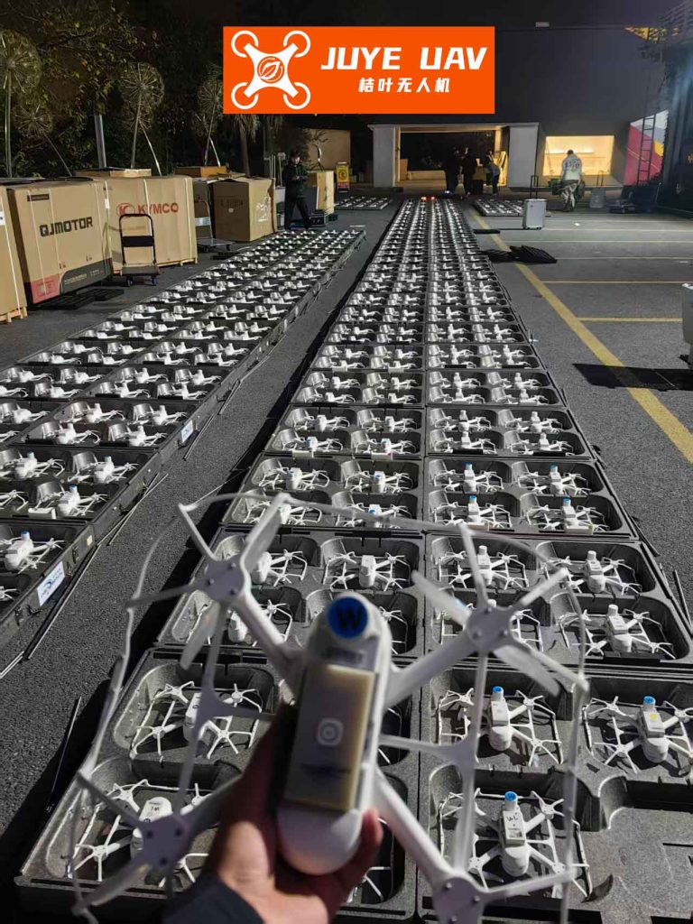
The average coverage rate over time further validates our method. As shown in the coverage plot, our algorithm achieved higher coverage faster compared to the non-BINN approach, indicating enhanced environmental adaptability. For a formation drone light show, this means drones can quickly adjust to changing conditions, such as wind or unexpected obstacles, ensuring a seamless performance. The integration of BINN allows drones to continuously update their neural activity maps, facilitating real-time decision-making that is crucial for complex aerial displays. In essence, the same principles that improve search efficacy also enhance the artistic precision and reliability of formation drone light shows, making them more resilient and captivating.
In conclusion, the proposed method combining BINN and MPC offers a robust solution for drone formation control, particularly suited for formation drone light shows. By leveraging bio-inspired neural networks, drones can dynamically perceive and map their environment, while MPC ensures precise and cooperative movements. The simulation results confirm that this approach increases search efficiency and environmental adaptability, key factors for successful aerial performances. Future work could extend this to 3D environments or incorporate more advanced machine learning techniques for even more dazzling formation drone light shows. As the demand for innovative entertainment grows, such intelligent systems will play a pivotal role in pushing the boundaries of what is possible with autonomous drone swarms.