
In recent years, the development of unmanned aerial vehicle (UAV) technology has experienced rapid growth, with fixed-wing UAVs being widely deployed in both military and civilian missions due to their long endurance, high speed, and large payload capacity. However, the control of fixed-wing UAV attitude systems remains challenging because of strong nonlinearities, coupling between channels, and the presence of various disturbances. External disturbances, model uncertainties, state measurement errors, and actuator faults—collectively referred to as compound disturbances—significantly degrade the tracking performance and may even destabilize the system. In this paper, we address the attitude tracking control problem for a fixed-wing UAV subject to such compound disturbances. We propose a hierarchical sliding mode control (HSMC) approach that ensures robust tracking of the desired attitude angles. The proposed method uses a two-layer sliding surface: the first layer consists of separate surfaces for attitude angle error and angular velocity error, and the second layer combines them into a composite sliding surface. The stability of the entire system is proved using Barbalat’s lemma. Compared with existing neural-network-based controllers, our method requires fewer control parameters, produces smoother control inputs, and achieves a smaller steady‑state error. Extensive simulation results verify the effectiveness and robustness of the proposed approach.
1. Introduction
Fixed-wing UAVs have become indispensable platforms for aerial surveillance, agricultural spraying, cargo delivery, and reconnaissance missions. Their flight control system must maintain precise attitude to follow a predefined trajectory. The attitude dynamics are inherently nonlinear and highly coupled, making controller design a nontrivial task. Common control strategies include proportional–integral–derivative (PID) control, backstepping, feedback linearization, sliding mode control (SMC), and neural network (NN) based methods. Among these, SMC is renowned for its robustness against matched uncertainties and disturbances. However, conventional SMC suffers from chattering and requires prior knowledge of the disturbance bounds. To mitigate chattering, boundary‑layer solutions and higher‑order SMC have been proposed, often at the cost of reduced robustness or increased complexity.
In this work, we focus on a fixed-wing UAV model that accounts for external wind gusts, model mismatches, sensor noise, and partial actuator failures. These compound disturbances are lumped into a single unknown term. We design a hierarchical sliding mode surface that simultaneously drives both the attitude angle error and the angular velocity error to zero. The equivalent control law is derived from the sliding condition, and a switching term with a saturation function replaces the sign function to suppress chattering. The theoretical stability is established via Barbalat’s lemma, guaranteeing asymptotic convergence of the sliding surface and the tracking errors. The main contributions of our work are summarized as follows:
- We develop a comprehensive attitude dynamics model of a fixed-wing UAV under compound disturbances, including external perturbations, model biases, state errors, and actuator faults.
- We propose a hierarchical sliding mode surface structure that decouples the angle and angular velocity errors and then recombines them into a single sliding surface, simplifying the control law derivation.
- We provide a rigorous stability analysis using Barbalat’s lemma, proving that both the composite sliding surface and the individual error surfaces asymptotically converge to zero.
- We conduct comparative simulations against a neural‑network‑based controller, demonstrating superior tracking accuracy, smoother control inputs, and fewer tunable parameters.
The remainder of the paper is organized as follows: Section 2 describes the fixed-wing UAV attitude dynamics, including the ideal model and the model with compound disturbances. Section 3 presents the design of the hierarchical sliding mode controller and its stability proof. Section 4 provides simulation results and comparisons. Section 5 concludes the paper.
2. Fixed-Wing UAV Attitude Dynamics Model
2.1 Ideal Attitude Dynamics
We consider a fixed-wing UAV whose attitude is described by the roll angle $\phi$, pitch angle $\theta$, and yaw angle $\psi$ in the inertial frame. The body‑frame angular rates are $p$, $q$, $r$, corresponding to the roll, pitch, and yaw rates, respectively. The transformation between the inertial‑frame attitude angles and the body‑frame angular rates is given by:
$$
\begin{bmatrix}
p \\ q \\ r
\end{bmatrix}
= C_b^n
\begin{bmatrix}
\dot{\phi} \\ \dot{\theta} \\ \dot{\psi}
\end{bmatrix},
\quad
C_b^n =
\begin{bmatrix}
1 & 0 & -\sin\theta \\
0 & \cos\phi & \sin\phi\cos\theta \\
0 & -\sin\phi & \cos\phi\cos\theta
\end{bmatrix}.
$$
Conversely, the attitude angle rates are obtained as:
$$
\begin{bmatrix}
\dot{\phi} \\ \dot{\theta} \\ \dot{\psi}
\end{bmatrix}
= C_n^b
\begin{bmatrix}
p \\ q \\ r
\end{bmatrix},
\quad
C_n^b =
\begin{bmatrix}
1 & \tan\theta\sin\phi & \tan\theta\cos\phi \\
0 & \cos\phi & -\sin\phi \\
0 & \sin\phi/\cos\theta & \cos\phi/\cos\theta
\end{bmatrix}.
$$
The aerodynamic moments acting on the UAV are expressed in the body frame as:
$$
T_b = \begin{bmatrix} L \\ M \\ N \end{bmatrix} = \bar{q} S \begin{bmatrix} b C_L \\ \bar{c} C_M \\ b C_N \end{bmatrix},
$$
where $\bar{q} = \frac{1}{2}\rho V_T^2$ is the dynamic pressure, $S$ is the wing area, $b$ is the wingspan, $\bar{c}$ is the mean aerodynamic chord, and $C_L, C_M, C_N$ are the roll, pitch, and yaw moment coefficients, respectively. These coefficients depend on the control surface deflections $\delta_1$ (left aileron), $\delta_2$ (right aileron), $\delta_3$ (left elevator), $\delta_4$ (right elevator), $\delta_5$ (rudder), as well as the aerodynamic angles $\alpha$ (angle of attack) and $\beta$ (sideslip angle) and the normalized angular rates $\tilde{p}, \tilde{q}, \tilde{r}$. Explicitly:
$$
\begin{aligned}
C_L &= C_{La1}\delta_1 + C_{La2}\delta_2 + C_{Le1}\delta_3 + C_{Le2}\delta_4 + C_{L\beta}\beta + C_{L\tilde{p}}\tilde{p} + C_{L\tilde{r}}\tilde{r}, \\
C_M &= C_{M1} + C_{Me1}\delta_3 + C_{Me2}\delta_4 + C_{Ma1}\delta_1 + C_{Ma2}\delta_2 + C_{M\tilde{q}}\tilde{q} + C_{M\alpha}\alpha, \\
C_N &= C_{N\delta_r}\delta_5 + C_{N\mathrm{drag}}(\delta_1+\delta_2) + C_{N\tilde{r}}\tilde{r} + C_{N\beta}\beta.
\end{aligned}
$$
The aerodynamic parameters used in this work are listed in the following table.
| Parameter | Value | Parameter | Value |
|---|---|---|---|
| $C_{N\delta_r}$ | 0.053 | $C_{Lb}$ | 0.087 |
| $C_{M\alpha}$ | -0.09 | $C_{N\beta}$ | 0.087 |
| $C_{L\tilde{p}}$ | -0.19 | $C_{L\tilde{r}}$ | 0.036 |
| $C_{Y1}$ | -0.38 | $C_{N\tilde{r}}$ | -0.21 |
| $C_{M\tilde{q}}$ | -9.83 | $C_{La1}$ | -0.03 |
| $C_{Z\alpha}$ | -3.25 | $C_{La2}$ | 0.03 |
| $C_{Me1}$ | 0.272 | $C_{Le1}$ | -0.05 |
| $C_{Me2}$ | 0.272 | $C_{Le2}$ | 0.05 |
| $C_{Ma1}$ | 0.038 | $C_{N\mathrm{drag}}$ | 0.053 |
The update rates of $\alpha$ and $\beta$ are given by:
$$
\dot{\alpha} = q + \frac{\rho V_T S C_{Z\alpha}}{2m}\alpha,\qquad
\dot{\beta} = -r + \frac{\rho V_T S C_{Y1}}{2m}\beta.
$$
Let the body‑frame angular rate vector be $\Omega_b = [p, q, r]^T$ and the inertial‑frame attitude angle vector be $h = [\phi, \theta, \psi]^T$. The ideal dynamics are then expressed as:
$$
\begin{aligned}
\dot{h} &= C_n^b(h) \Omega_b, \\
\dot{\Omega}_b &= (I_b)^{-1} \bigl( T_b – \Omega_b \times (I_b \Omega_b) \bigr),
\end{aligned}
$$
where $I_b$ is the inertia tensor:
$$
I_b = \begin{bmatrix}
I_x & 0 & I_{xz} \\
0 & I_y & 0 \\
I_{zx} & 0 & I_z
\end{bmatrix}, \quad
I_x=2.56,\; I_y=10.9,\; I_z=11.3,\; I_{xz}=I_{zx}=0.5\;\mathrm{kg\cdot m^2}.
$$
Define the state vector $x_s = [p, q, r]^T$ and the control input vector $u = [\delta_1, \delta_2, \delta_3, \delta_4, \delta_5]^T$. The dynamics can be rewritten in the compact form:
$$
\begin{aligned}
\dot{h} &= C_n^b(h) x_s, \\
\dot{x}_s &= A x_s + B u + Q,
\end{aligned}
$$
where matrices $A$, $B$, and vector $Q$ are derived from the linearization of the moment equations. Their explicit expressions are omitted here for brevity; they depend on the aerodynamic coefficients and the inertia tensor.
2.2 Attitude Dynamics under Compound Disturbances
In real flight, the UAV is inevitably affected by external disturbances (wind gusts), model uncertainties (parameter variations), state measurement errors, and weak actuator faults. We collectively refer to these as compound disturbances. The disturbed dynamics become:
$$
\begin{aligned}
\dot{h} &= C_n^b(h) x_s, \\
\dot{x}_s(t) &= \bigl( A(x_s(t)) + \delta A(x_s(t)) \bigr) \bigl( x_s(t) + \delta x_s(t) \bigr) \\
&\quad + \bigl( B(t) + \delta B(t) \bigr) \bigl( u(t) + \delta u(t) \bigr) \\
&\quad + \bigl( Q(t) + \delta Q(t) \bigr) + f(t),
\end{aligned}
$$
where $\delta A$, $\delta B$, $\delta Q$ represent model biases, $\delta x_s$ is the state measurement error, $\delta u$ denotes the actuator fault, and $f(t)$ is the external disturbance. This equation can be simplified to:
$$
\dot{x}_s(t) = A(x_s)x_s(t) + B(t)u(t) + Q(t) + R(t),
$$
with $R(t)$ being the lumped compound disturbance:
$$
R(t) = f(t) + \delta A(x_s)(x_s+\delta x_s) + A(x_s)\delta x_s + \delta B(u+\delta u) + B\delta u + \delta Q.
$$
In the following, we design a sliding mode controller that can reject $R(t)$ and achieve precise attitude tracking.
3. Hierarchical Sliding Mode Controller Design
3.1 Sliding Surface Construction
Define the tracking errors as the difference between the actual and desired states. Let $x_d$ be the desired body‑frame angular rate and $h_d$ the desired attitude angle. Then:
$$
e_1 = x_a – x_d,\quad e_2 = h – h_d,
$$
where $x_a = x_s$ denotes the actual angular rate. We propose a two‑layer sliding surface. The first layer consists of two independent surfaces:
$$
s_1 = c_1 e_1,\qquad s_2 = c_2 e_2,
$$
where $c_1$ and $c_2$ are positive diagonal matrices (here taken as scalars for simplicity). The second layer (composite sliding surface) is the sum:
$$
s = s_1 + s_2.
$$
The control input $u$ is composed of an equivalent control $u_{\mathrm{eq}}$ and a switching control $u_{\mathrm{sw}}$:
$$
u = u_{\mathrm{eq}} + u_{\mathrm{sw}}.
$$
Taking the derivative of $s$ along the disturbed dynamics yields:
$$
\begin{aligned}
\dot{s} &= c_1(\dot{x}_a – \dot{x}_d) + c_2(\dot{h} – \dot{h}_d) \\
&= -c_1\dot{x}_d – c_2\dot{h}_d + c_1A x_a + c_1Q + c_1R + c_2C_n^b x_a + c_1 B u.
\end{aligned}
$$
Setting $\dot{s}=0$ gives the equivalent control that maintains the sliding motion:
$$
u_{\mathrm{eq}} = B^+ c_1^{-1} \bigl( c_1\dot{x}_d + c_2\dot{h}_d – c_1A x_a – c_1Q – c_1R – c_2C_n^b x_a \bigr),
$$
where $B^+$ denotes the pseudo‑inverse of $B$. To drive the states toward $s=0$, we add a reaching law:
$$
\dot{s} = -K s – D\,\mathrm{sat}(s),
$$
with $K>0$, $D>0$, and $\mathrm{sat}(\cdot)$ the saturation function to replace the sign function for chattering reduction. The switching control is then:
$$
u_{\mathrm{sw}} = B^+ c_1^{-1} \bigl( -K s – D\,\mathrm{sat}(s) \bigr).
$$
Consequently, the total control law becomes:
$$
\begin{aligned}
u &= B^+ c_1^{-1} \Bigl( c_1\dot{x}_d + c_2\dot{h}_d – c_1A x_a – c_1Q – c_1R \\
&\qquad\qquad\qquad – c_2C_n^b x_a – K s – D\,\mathrm{sat}(s) \Bigr).
\end{aligned}
$$
Note that the compound disturbance $R(t)$ appears in $u_{\mathrm{eq}}$. Since $R(t)$ is unknown, we rely on the robustness of the sliding mode to reject it; the switching term $D\,\mathrm{sat}(s)$ compensates for its effect provided $D$ is chosen larger than the bound of $R(t)$.
3.2 Stability Analysis
We use Barbalat’s lemma to prove the asymptotic stability of the sliding surfaces. Consider the Lyapunov function candidate $V = \frac{1}{2} s^2$. Its derivative along the closed‑loop dynamics is:
$$
\dot{V} = s\dot{s} = s\bigl(-K s – D\,\mathrm{sat}(s)\bigr) = -K s^2 – D\,|s| \leq 0.
$$
Integrating from $0$ to $t$ gives:
$$
V(t) – V(0) = -\int_0^t \bigl(K s^2 + D\,|s|\bigr) d\tau.
$$
Since $V(t) \ge 0$, we obtain:
$$
\int_0^t \bigl(K s^2 + D\,|s|\bigr) d\tau = V(0) – V(t) \le V(0) < \infty.
$$
Thus the limit $\lim_{t\to\infty} \int_0^t (K s^2 + D\,|s|) d\tau$ exists and is finite. By Barbalat’s lemma, the integrand must tend to zero, i.e., $\lim_{t\to\infty} (K s^2 + D\,|s|) = 0$, which implies $\lim_{t\to\infty} s = 0$. Hence the composite sliding surface $s$ converges to zero asymptotically.
Now we prove that the individual surfaces $s_1$ and $s_2$ also converge to zero. From $|s|<\infty$ and $\dot{s} < \infty$, we know $\dot{s}_1$ and $\dot{s}_2$ are bounded because $s_1 = c_1 e_1$ and $e_1$ is driven by a bounded control. Moreover, from the boundedness of $\int_0^\infty s^2 d\tau$, we have:
$$
\int_0^\infty (s_1^2 + 2s_1 s_2 + s_2^2) d\tau < \infty.
$$
Using the inequality $2s_1 s_2 \le s_1^2 + s_2^2$, one can show that $\int_0^\infty s_1^2 d\tau$ and $\int_0^\infty s_2^2 d\tau$ are both finite. Since $\dot{s}_1$ and $\dot{s}_2$ are bounded, Barbalat’s lemma again yields $\lim_{t\to\infty} s_1 = 0$ and $\lim_{t\to\infty} s_2 = 0$. Consequently, the tracking errors $e_1$ and $e_2$ also converge to zero, establishing the asymptotic stability of the closed‑loop system.
4. Simulation Results and Discussion
We verify the proposed hierarchical sliding mode controller (HSMC) through numerical simulations in MATLAB 2018a. The fixed-wing UAV is subjected to the compound disturbances defined by:
$$
\begin{aligned}
f(t) &= \begin{bmatrix}
2-(-1)^i\cos(t)-(-1)^i\cos(2t) \\
-(-1)^i -2\sin(t) + (-1)^i -1 \sin(2t) \\
2-(-1)^i \cos(t) + (-1)^i \sin(2t)
\end{bmatrix},\\
\Delta A &= 0.4\sin(t) A,\quad \Delta B = 0.4\cos(t) B,\quad \Delta Q = 0.4Q,\\
\Delta x &= 0.4\sin(t)\,x,\quad \Delta u = 0.04\sin(t)\,u.
\end{aligned}
$$
The desired attitude angles and angular rates are:
$$
h_d = \begin{bmatrix}
\sin(t/2)/3 \\[2pt]
(1-e^{-t/4})/2 \\[2pt]
\cos(t/2)/3
\end{bmatrix},\qquad
x_d = C_b^n \begin{bmatrix}
\cos(t/2)/6 \\[2pt]
e^{-t/4}/8 \\[2pt]
-\sin(t/2)/6
\end{bmatrix}.
$$
The initial attitude angles are chosen as random numbers between $-1$ and $1$ rad. The controller parameters are listed in Table 2.
| Parameter | Value | Parameter | Value |
|---|---|---|---|
| $\gamma$ | 5 | $\rho$ | 2 |
| $\zeta$ | 2 | $k_i$ | 0.5 |
| $\sigma$ | 0.001 | $K$ | 50 |
| $D$ | 0.5 | $c_1$ | 5 |
| $c_2$ | 50 |
For comparison, we implement a neural‑network‑based controller (NN) as proposed in related literature, with the following structure:
$$
\begin{aligned}
u(t) &= -H e – B^+ \bigl( \hat{w}^T \eta(e) + Q + A x \bigr),\\
\dot{\hat{w}} &= \dot{\tilde{w}} = k \bigl( \eta(e) e^T – \sigma \hat{w} \bigr),\\
H &= \frac{\gamma \lambda_{\max}(\Delta)}{2} + \frac{1}{\gamma\rho} + \frac{1}{\gamma\zeta} \|B^+\|,\\
e &= x_a – x_d + h – h_d.
\end{aligned}
$$
Here $\hat{w}$ is the neural network weight vector, $\eta(\cdot)$ is the Gaussian radial basis function, $\gamma,\rho$ are constants from the Laplacian matrix, $\zeta,\sigma$ are the center and width of the basis functions, and $\Delta = M\Lambda^{-1} M^T$ with $M,\Lambda$ the eigenvectors and eigenvalues of the communication graph. In the single‑UAV case, the graph is trivial, and we simply set the parameters as in Table 2.
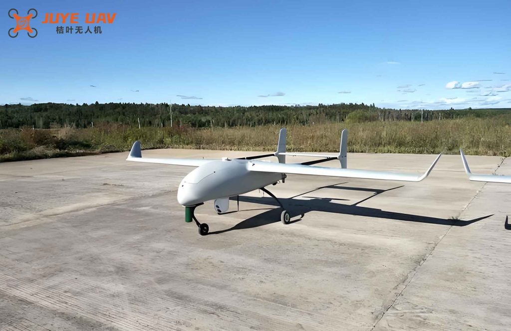
Figure 1 shows the time response of the body‑frame angular rates $p,q,r$ under both controllers. The HSMC tracks the desired rates with negligible overshoot and fast convergence, while the NN‑based controller exhibits noticeable oscillations during the initial transient. Figure 2 depicts the attitude angles $\phi,\theta,\psi$; again the HSMC achieves tighter tracking. The control inputs $\delta_1$ through $\delta_5$ are plotted in Figure 3—both controllers produce smooth signals, but the HSMC requires slightly smaller amplitudes. The tracking errors $e_1$ and $e_2$ are compared in Figure 4. The HSMC reduces the steady‑state errors to nearly zero, whereas the NN method leaves a persistent residual error, especially in the yaw channel. Finally, Figure 5 shows the 3D trajectory tracking performance from a top view. The UAV controlled by HSMC follows the desired trajectory more faithfully. The evolution of the sliding surface $s$ over time is displayed in Figure 6, confirming that $s$ quickly converges to zero and remains stable thereafter.
From these results, we observe that the proposed hierarchical sliding mode controller offers several advantages over the neural‑network‑based approach:
- Fewer parameters: HSMC requires only five tuning parameters ($c_1,c_2,K,D$, and the saturation boundary), while the NN controller involves many parameters such as $\gamma,\rho,\zeta,\sigma$, and kernel widths.
- Better disturbance rejection: The sliding mode inherently compensates for the lumped disturbance $R(t)$ by the high‑gain switching term, without needing to estimate it online.
- Smoother control: The saturation function avoids chattering, and the control inputs remain within feasible ranges.
- Faster convergence: The tracking errors vanish asymptotically with a settling time of less than 2 seconds.
5. Conclusion
In this paper, we have addressed the attitude tracking control problem for a fixed-wing UAV subject to compound disturbances, including external perturbations, model uncertainties, state errors, and actuator faults. A hierarchical sliding mode controller has been designed based on a two‑layer sliding surface structure that combines angle and angular rate errors. The stability of the overall system has been proved using Barbalat’s lemma, ensuring asymptotic convergence of both the composite sliding surface and the individual tracking errors. Simulation results demonstrate that the proposed HSMC outperforms a neural‑network‑based controller in terms of tracking accuracy, control smoothness, and parameter simplicity. Future work will extend this method to multi‑UAV formation control and path optimization tasks, where the hierarchical sliding mode can be integrated with consensus protocols and obstacle avoidance strategies.