
In recent years, the rapid advancement of small tactical unmanned aerial vehicles (UAVs), both fixed-wing and rotary-wing, has made saturation attacks based on drone swarms a primary threat to existing air defense systems. Traditional countermeasures against such anti-drone scenarios are broadly categorized into soft kills, such as deception jamming, laser suppression, and high-power microwave damage, and hard kills, such as anti-aircraft artillery and short-range air defense missiles. However, soft-kill methods are susceptible to complex electromagnetic environments, have limited effectiveness against UAVs with specific configurations or strong anti-jamming capabilities, and often suffer from insufficient effective range. Hard-kill methods, on the other hand, face significant limitations, including low cost-effectiveness, high risks of collateral damage, and insufficient flexibility in dealing with highly maneuverable targets. In contrast, interceptor UAVs, with their low cost, high maneuverability, rapid response capabilities, and crucially, the potential for swarm cooperative operations, have emerged as an ideal solution to modern anti-drone swarm threats. Nonetheless, the core challenge in effectively leveraging interceptor UAV swarms lies in efficiently solving the dynamic, large-scale target allocation problem in anti-drone operations. This involves real-time optimal matching of our limited and variably state interceptor UAV resources with numerous, high-speed, maneuvering enemy UAV targets of varying threat levels in highly dynamic battlefield environments. The goal is to maximize overall interception effectiveness while minimizing operational costs under multiple strong constraints, such as kill probability, time windows, resource consumption, and collision avoidance. This problem is characterized by high dimensionality, strong constraints, multi-objective nature, dynamic time-varying conditions, and NP-hard complexity, making traditional optimization methods inadequate for real-time solutions.
Given the complexity and real-time requirements of the anti-drone problem, intelligent optimization algorithms, represented by the Genetic Algorithm (GA), have shown significant potential and application prospects in solving dynamic target allocation for anti-drone swarms, owing to their powerful global search capabilities, adaptability to complex constraints, and inherent parallel processing mechanisms. Recent research has made positive progress; however, current studies on target allocation for anti-drone swarms remain insufficient, particularly regarding the use of interceptor UAVs to counter UAV swarms. Therefore, research in this anti-drone context holds considerable value.
As scholars delve deeper into genetic algorithms, issues such as low initial population diversity, slow convergence speed, and poor solution quality have been identified in solving anti-drone swarm target allocation problems. Proper initialization of genetic algorithms is a powerful means to address these issues. In recent years, the academic community has conducted multi-dimensional improvements to GA initialization. Methods such as using prior human knowledge as heuristic information to assist population initialization, employing artificial bee colony solutions as initial populations for NSGA-III, generating diverse initial subpopulations in parallel via multiple processors, and utilizing k-means techniques for initialization have been proposed. However, these methods generally suffer from high computational complexity, insufficient adaptability to high dimensions, strong parameter sensitivity, and limitations in the uniformity and traversal of solution space distribution. Especially when dealing with high-dimensional optimization problems, the quality and diversity assurance mechanisms of initial populations are notably inadequate, hindering further algorithm performance improvement.
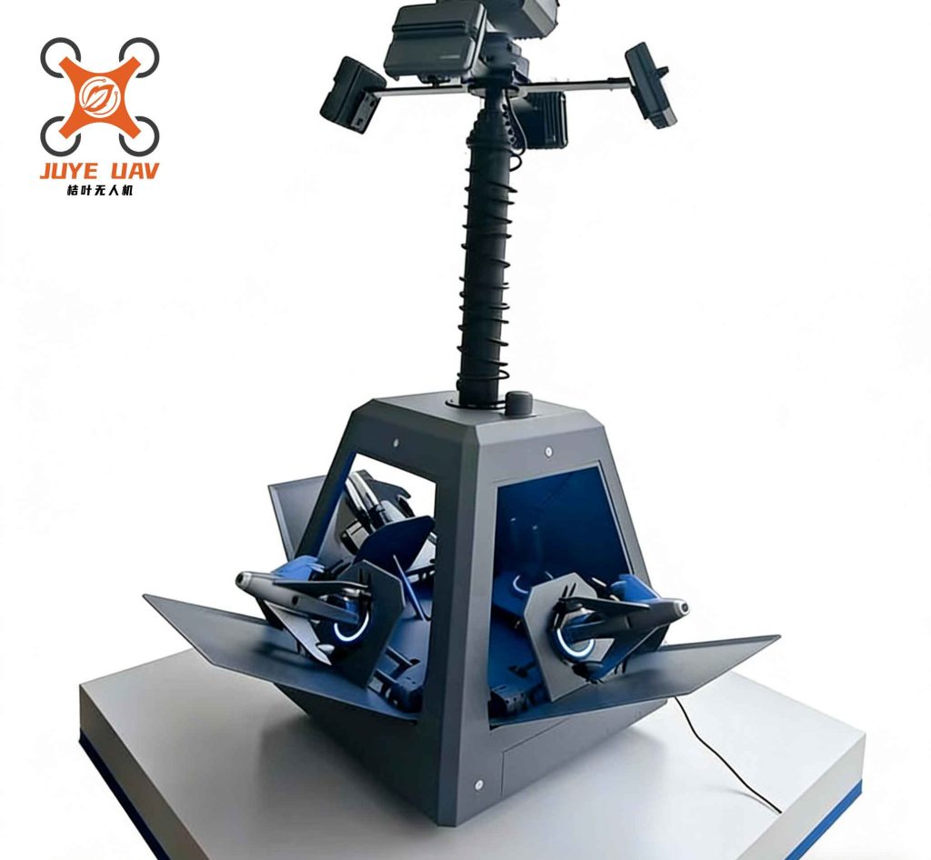
To address these issues, I propose a chaos-enhanced hybrid genetic algorithm and simulated annealing (CE-HGASA) that incorporates dual Logistic chaotic mapping initialization. This algorithm is designed to enhance population diversity and improve convergence performance in anti-drone target allocation. Furthermore, within the context of anti-drone swarm target allocation, I establish a multi-constraint target allocation mathematical model that maximizes system interception effectiveness and minimizes overall interception costs, incorporating dynamic trajectory prediction of targets. By applying the proposed CE-HGASA algorithm to solve this model, I aim to verify its feasibility. Experimental results demonstrate that CE-HGASA reduces the average number of generations required to converge to the optimal solution by 36% compared to traditional genetic algorithms and by 20% compared to the baseline algorithm without chaotic mapping, with convergence generation variance an order of magnitude lower than that of traditional GA. This algorithm effectively improves solution speed and stability, providing an efficient and reliable approach for dynamic real-time target allocation in anti-drone swarm operations.
Algorithm Design: Enhanced Hybrid Genetic Annealing Approach
The traditional genetic algorithm employs random initialization for population generation, which can lead to population clustering, causing the algorithm to easily fall into local optima. In the proposed CE-HGASA algorithm, I introduce dual Logistic mapping to generate a highly diverse initial population, construct a fitness function based on kill rate and cost-effectiveness ratio, and achieve comprehensive optimization through Pareto sorting.
The flowchart of the CE-HGASA algorithm is as follows. The algorithm design is described against the backdrop of target allocation problems for the defending side in anti-drone operations.
Encoding
To avoid the normalization of decision variables required by real-number encoding and potential conversion errors, I use binary encoding. Specifically, existing defender UAVs in the formation are denoted as i (i = 1, 2, …, n), and UAVs to be engaged are denoted as j (j = 1, 2, …, m). The final allocation result is recorded as an i × j dimensional matrix U = [u_{ij}], where u_{ij} is an element in the matrix. u_{ij} = 1 indicates that the i-th defender UAV is assigned to the j-th target, and u_{ij} = 0 indicates that the j-th attacker UAV is not assigned to the i-th defender UAV. The matrix U is compressed into a one-dimensional vector in row order, recorded as a chromosome in the genetic algorithm, with each gene on the chromosome corresponding to a Boolean value indicating whether a defender UAV attacks a target. All chromosomes constitute the population in the genetic algorithm.
Population Initialization
The CE-HGASA algorithm employs a dual Logistic mapping strategy for population initialization to enhance the traversal and randomness of the initial population. This process consists of two stages: first, using basic Logistic mapping to preliminarily evolve the current sequence value z_k to obtain an intermediate variable x_k, expressed as:
$$x_k = \mu z_k (1 – z_k), \quad z_k \in (0,1)$$
Based on this, the intermediate variable x_k is used as input, and the same rule of Logistic mapping is applied again to obtain the next iteration’s sequence value z_{k+1}. The second mapping and the entire dual mapping process are mathematically represented as:
$$z_{k+1} = \mu \cdot x_k (1 – x_k)$$
$$z_{k+1} = \mu [\mu z_k (1 – z_k)] \cdot (1 – \mu z_k (1 – z_k))$$
where μ is the mapping parameter, ranging from [0, 4], and when 3.569945 ≤ μ ≤ 4, the Logistic mapping exhibits chaotic properties with good traversal. k is the mapping iteration number, with the total number determined by (population size × chromosome length), where population size is the number of chromosomes in a population, and chromosome length is i × j. z_k represents the current iteration’s sequence value; x_k represents the output value of the first mapping, used as the input for the second mapping. z_{k+1} represents the final output value of the dual mapping.
Since binary encoding is used, and Logistic mapping generates continuous value sequences, a threshold r = 0.5 is set. When z_k ≥ r, the current sequence value is taken as 1; when z_k < r, it is taken as 0. Subsequently, the final binary sequence obtained through dual mapping processing is divided into groups based on population size and chromosome length, with each group forming a chromosome, thereby constructing the initial population. This dual mapping mechanism, through nonlinear superposition effects, effectively mitigates the probability density distribution distortion phenomenon (i.e., endpoint clustering effect) present in the original Logistic mapping at value domain boundary regions, enhancing the traversal uniformity of the sequence.
Fitness Function
Based on the current moment information of attacker UAVs, defender UAVs have different interception hit rates and kill rates against attacker UAV targets. In the algorithm, an interception success rate matrix P = [p_{ij}] is used, where p_{ij} represents the success rate of the i-th defender UAV intercepting the j-th attacker UAV:
$$p_{ij} = R_{h}^i R_{da}^i$$
where R_{h}^i is the hit rate of the i-th defender UAV intercepting the j-th attacker UAV, and R_{da}^i is the kill rate of the i-th defender UAV striking the j-th attacker UAV.
Let the cost of the i-th defender UAV intercepting the j-th attacker UAV be c_{ij}, and the threat level of the j-th attacker UAV be ω_{ij}. Then the cost-effectiveness ratio f_{ij} for interception can be expressed as:
$$f_{ij} = \frac{\omega_{ij}}{c_{ij}}$$
The objective function maximizing interception rate and minimizing interception cost is:
$$E = \max \sum_{i=1}^{M} \sum_{j=1}^{N} [(\alpha p_{ij} + \gamma f_{ij}) u_{ij}]$$
where E is the objective function aimed at maximizing overall interception effectiveness while minimizing interception cost. Additionally, before each iteration, the algorithm calculates the minimum fitness value of the population and sets 120% of it as a dynamic threshold. All individuals with fitness values below this threshold are regenerated randomly, thereby introducing new solutions and significantly enhancing population diversity.
Selection Operation
Based on the fitness function, the fitness values of all chromosomes in each iteration are calculated and sorted. During iteration, an elite preservation strategy is used: each iteration replaces the bottom 20% of chromosomes with the currently preserved best chromosomes, i.e., replacing the 20% least fit chromosomes with the fittest chromosomes, driving the population to evolve toward better adaptation to the environment.
Crossover Operation
In the CE-HGASA algorithm, crossover operation employs multi-point crossover combined with an adaptive crossover rate strategy. The specific process is: randomly select two parent chromosomes P1 and P2 from the population, generate m non-repeating crossover points within the chromosome length range (m ∈ [2, 5]), divide the chromosome into m + 1 gene segments, and alternately exchange parent gene segments to generate offspring. For example, when m = 4, crossover points divide the chromosome into 5 segments (S1, S2, S3, S4, S5). Offspring C1 inherits S1, S3, and S5 from P1 and S2 and S4 from P2, while offspring C2 inherits S1, S3, and S5 from P2 and S2 and S4 from P1. This design enhances solution space perturbation capability by increasing gene fragment exchange times, avoiding limitations of single-point crossover locality.
To dynamically balance global exploration and local development capabilities, the crossover rate P_c is adaptively adjusted based on population diversity. Diversity is quantified through population gene entropy H:
$$H = -\sum_{i=1}^{L} \sum_{j \in \{0,1\}} p_{ij} \log_2(p_{ij})$$
where L is the chromosome length; p_{ij} represents the probability that the i-th gene locus takes value j. The crossover rate adjustment rules are as follows:
When population gene entropy is below a set threshold (60% of initial gene entropy), the population is judged to have a degradation trend. At this time, the crossover rate is increased to near 0.95 to promote new solution generation by enhancing gene recombination intensity, avoiding the algorithm falling into local optima. When population gene entropy is at a high level (above the threshold), the crossover rate is reduced to near the lower limit to reduce damage to the gene structure of excellent individuals, ensuring stable inheritance of elite solutions. The specific calculation process is as follows:
$$P_c = \begin{cases}
P_{c,\max} – a (H – H_{\text{threshold}}), & \text{if } H < H_{\text{threshold}} \\
P_{c,\min} – b (H_{\text{threshold}} – H), & \text{otherwise}
\end{cases}$$
where P_{c,\max} represents the upper limit of crossover rate, defined as 0.95; P_{c,\min} represents the lower limit, defined as 0.70; a and b are adjustment coefficients, with a = 0.1, b = 0.05; H_{\text{threshold}} is the gene entropy threshold, defined as 0.6 times the initial population gene entropy.
Mutation Operation
In CE-HGASA, the initial probability of mutation operation is set first, and before each mutation, a random number between 0 and 1 is generated. If this number is less than the current mutation probability, mutation operation is performed. To control mutation intensity and enhance population diversity, a non-uniform mutation strategy is adopted. The perturbation amplitude is controlled by:
$$\Delta(k) = \left(1 – \frac{k}{K}\right)^b$$
where Δ(k) is the perturbation intensity to mutation probability at the k-th iteration; k represents the current iteration number; K is the maximum iteration count; b is the decay coefficient, used to control the probability decline speed, set to 2 in this experiment.
The mutation probability decay function is:
$$y_k = y_{\min} + \Delta(k) (y_{\max} – y_{\min})$$
where y_k represents the current iteration mutation probability; y_{\min} represents the final mutation probability, set to 0.1; y_{\max} represents the initial mutation probability, set to 0.3. The mutation rate decreases with iterations, helping to increase mutation probability early to expand search range and increase solution space coverage, and reduce mutation probability later to enhance local convergence.
Simulated Annealing Mechanism
In the proposed algorithm, the simulated annealing mechanism is embedded after mutation operation to decide whether to accept newly generated individuals. The specific implementation process is as follows: first, after each generation of genetic operations, the fitness value of the new individual is calculated and compared with its corresponding parent individual’s fitness. If the new individual’s fitness is better than the parent’s, the new individual is directly accepted, replacing the parent individual in the next generation population. If the new individual’s fitness is worse, according to the simulated annealing criterion, it is accepted with a certain probability, calculated by:
$$P_{SA} = \exp\left(\frac{\Delta E}{T}\right)$$
where ΔE = E_{\text{new}} – E_{\text{parent}} represents the fitness difference; T is the current annealing temperature. The annealing temperature T gradually decreases with iteration number k, typically using the following decay formula:
$$T_{k+1} = \lambda \times T_k$$
where λ is the cooling coefficient, ensuring temperature slowly decreases with iteration, gradually reducing the probability of accepting inferior solutions, enhancing algorithm stability and convergence. To ensure early frequent acceptance of inferior solutions, expanding search range and escaping local optima, a high initial temperature T_0 is set at algorithm initialization. As iterations proceed, temperature gradually decreases, making search converge near excellent solutions. This mechanism effectively introduces randomness and global search capability on the basis of genetic algorithm, improving algorithm performance in multi-objective kill rate and cost-effectiveness ratio optimization.
Algorithm Flow
The algorithm employs a core strategy of “global rapid positioning + local fine optimization.” Through dual-layer Logistic chaotic mapping to uniformly scatter points in solution space, it addresses the issue of insufficient initial population diversity in traditional genetic algorithms. It integrates Pareto dominance relations to construct a fitness function, transforming maximization of interception effectiveness and minimization of cost into multi-objective optimization driving forces. Adaptive crossover/mutation operators are used to dynamically balance exploration and exploitation, embedding the simulated annealing Metropolis criterion to probabilistically accept inferior solutions, avoiding premature convergence. Finally, through elite retention and termination threshold dual mechanisms, the algorithm ensures output of high-stability optimal target allocation solutions within limited iterations. The flow design emphasizes a four-stage closed loop: “chaotic initialization – multi-objective evaluation – adaptive evolution – annealing selection,” achieving efficient solution of target allocation for UAV swarms in dynamic battlefield environments. Specific implementation steps are as follows:
- Initialize genetic algorithm parameters and population: set population size NP, maximum iteration count K, generate uniformly distributed initial population via dual Logistic mapping.
- Calculate individual fitness and sort: based on multi-objective function (maximize interception effectiveness, minimize interception cost), calculate fitness values of all chromosomes, combining target threat level, interception success rate, cost matrix, and dynamic trajectory prediction. Sort from high to low fitness, retain top 80% high-quality individuals.
- Retain top 20% optimal individuals directly into next generation. Then, randomly pair remaining individuals, exchange gene segments via 2 to 5 crossover points.
- For individuals with fitness below threshold (120% of current minimum fitness), randomly flip gene bits with decreasing probability (high early, low late) to complete mutation, enhancing local search capability.
- For mutated offspring individuals, calculate probability to accept inferior solutions using the simulated annealing formula, with temperature calculated via decay formula (T_0 = 100, decaying with iterations), avoiding algorithm falling into local optima.
- If current iteration count or fitness change for 20 consecutive generations is less than 1%, output optimal allocation matrix (chromosome); otherwise, increment iteration number k by 1, jump to step 2 to update population and repeat iteration.
Mathematical Model for Anti-Drone Combat Target Allocation
To verify the feasibility and superiority of the proposed algorithm in anti-drone swarm defense missions, I construct the following mathematical model. In anti-drone swarm defense missions, the challenge faced by the defending side is: under high-density, high-speed attacker UAV swarm threats, based on limited defense resources, achieve reasonable and rapid target allocation to maximize overall interception effectiveness. This process must not only consider interception success rate but also balance multiple factors such as target threat level and own weapon consumption. Since enemy target motion trajectories are highly dynamic, during mission allocation decisions, their future states must be predicted in real-time to improve the effectiveness and accuracy of interception decisions. To this end, let the number of defender UAVs be M, and the number of attacker incoming targets be N. Define the mission allocation strategy of defenders to targets as a decision matrix:
$$U = [u_{ij}], \quad u_{ij} \in \{0,1\}$$
where u_{ij} = 1 indicates the i-th defender UAV targets the j-th attacker UAV. To accurately evaluate the effectiveness of mission allocation, the following matrices are constructed:
- Interception success rate matrix P = [p_{ij}], representing the probability of defender UAV i successfully intercepting target j.
- Threat level matrix W = [w_{ij}], representing the threat weight of target j to the defender system. Threat weight is derived from assessment based on distance of attacker UAV from defense target, flight speed, flight direction, and tactical level of attacker UAV, weighted accordingly:
$$w_{ij} = w_1 \cdot d_j + w_2 \cdot \nu_j + w_3 \cdot T_j$$
where d_j represents the reciprocal of distance between attacker UAV j and defender key area; ν_j represents the current velocity vector of attacker UAV j; T_j represents the tactical level of attacker UAV; w_1, w_2, w_3 are weight coefficients for each threat factor. - Interception cost matrix C = [c_{ij}], representing the cost consumed by defender UAV i to intercept target j (i.e., ammunition, distance, and mission time), expressed as:
$$c_{ij} = \alpha \cdot A_i + \beta \cdot D_{ij} + \delta \cdot t_{ij}$$
where A_i represents the cost of defender UAV i; D_{ij} represents the flight distance used by defender UAV i to successfully intercept attacker UAV j; t_{ij} represents the total mission time of defender UAV i from takeoff to task completion; α, β, δ are weight coefficients, reflecting the relative importance of each factor to mission cost.
Additionally, considering dynamic trajectory prediction of target j, let the state of target j at time t be:
$$S_j(t) = [X_j(t), \nu_j(t)]$$
where X_j(t) ∈ ℝ³ is the target’s current position; ν_j(t) ∈ ℝ³ is its velocity vector. To enhance real-time performance of mission allocation, a predicted trajectory function is constructed:
$$X_j(t + \Delta t) = f_j(x_j(t), v_j(t), \Delta t)$$
This function performs short-term dynamic prediction of target trajectory, ensuring interception decisions are based on the target’s future state rather than current static position. Meanwhile, the calculation of interception success rate p_{ij} relies on dynamic prediction results, i.e., the success probability p_{ij} of UAV i intercepting target j needs to combine predicted target position, speed, and the UAV’s own interception capabilities (such as range, maneuverability), by dynamically adjusting interception path and time window, improving actual hit rate. Based on the above, an optimization objective function is established to maximize overall interception effectiveness while minimizing interception cost, combined with target dynamic trajectory prediction to improve interception success rate. To ensure feasibility of mission allocation, the following constraints are imposed:
$$\sum_{i=1}^{M} u_{ij} \leq \gamma_j, \quad \forall j = 1, \dots, N$$
$$\sum_{j=1}^{N} u_{ij} \cdot c_{ij} \leq R_i, \quad \forall i = 1, \dots, M$$
where γ_j represents the maximum allowed interception times for target j. The first constraint is the task uniqueness constraint, requiring each enemy target to be intercepted by at most a certain number of UAVs. The second constraint is the resource upper limit constraint, requiring the total resource consumption of each UAV during mission execution not to exceed its maximum carrying capacity.
Simulation Experiments and Analysis
To effectively verify the performance of the improved genetic algorithm, ablation experiments are conducted comparing CE-HGASA, traditional genetic algorithm (GA), and hybrid genetic algorithm and simulated annealing (HGASA) without chaotic mapping, from the perspectives of operational efficiency and algorithm robustness. To ensure scientificity and reliability of comparison, the operational parameters of target UAVs and own UAVs are kept consistent. The experiment assumes that the enemy uses Springknife-600 drone swarms to launch saturation attacks on the defense area, while the defender mobilizes own UAVs based on attacker drone swarm information for interception counterattacks. Software uses the Python open-source evolutionary algorithm toolbox Geatpy2 for algorithm development. Hardware configuration is Intel(R) Core(TM) i5-1035G1 CPU, clock speed 1.19 GHz, memory 8 GB.
Experiment 1: Logistic Mapping Ablation Experiment
To investigate the impact of Logistic mapping initialization on the proposed algorithm, a 20 vs. 20 drone swarm confrontation mode is used for experimentation. Assuming in an air defense operation, defender UAVs are deployed within a radius of 50 meters centered at the origin, and attacker formation initial positions are random points within [0,0,500] to [1000,1000,1000] to mimic the scenario of rapid attacker UAV approach difficult to detect in advance. Attacker UAV initial positions, initial velocities, and threat levels are as follows:
| Number | Initial Coordinates | Initial Velocity | Threat Level |
|---|---|---|---|
| 1 | [725, 541, 836] | 10 | 0.35 |
| 2 | [831, 599, 545] | 10 | 0.43 |
| 3 | [616, 806, 696] | 10 | 0.35 |
| 4 | [680, 818, 870] | 10 | 0.28 |
| 5 | [831, 575, 812] | 10 | 0.32 |
| 6 | [915, 730, 971] | 10 | 0.21 |
| 7 | [884, 752, 645] | 10 | 0.31 |
| 8 | [621, 544, 672] | 10 | 0.44 |
| 9 | [887, 553, 594] | 10 | 0.38 |
| 10 | [786, 765, 711] | 10 | 0.32 |
| 11 | [507, 641, 579] | 10 | 0.47 |
| 12 | [673, 552, 946] | 10 | 0.32 |
| 13 | [693, 901, 985] | 10 | 0.21 |
| 14 | [948, 627, 772] | 10 | 0.29 |
| 15 | [989, 769, 696] | 10 | 0.26 |
| 16 | [636, 824, 721] | 10 | 0.33 |
| 17 | [956, 952, 843] | 10 | 0.18 |
| 18 | [621, 556, 974] | 10 | 0.32 |
| 19 | [978, 686, 980] | 10 | 0.20 |
| 20 | [918, 627, 573] | 10 | 0.35 |
Parameter settings for the three algorithms are as follows:
| Algorithm | CE-HGASA | GA | HGASA |
|---|---|---|---|
| Iterations | 50 | 50 | 50 |
| Population | 200 | 200 | 200 |
| Crossover Rate | 0.70–0.95 | 0.90 | 0.70–0.95 |
| Mutation Rate | 0.30–0.01 | 0.05 | 0.30–0.01 |
| Annealing Temperature | 300 | None | 300 |
Algorithm convergence speed is quantified by the number of iterations required to converge to the optimal solution: the smaller this indicator, the shorter the solution time and higher efficiency under the same computational scale. The fitness value is the objective function value. Since the optimization goal is to maximize the objective function, higher fitness indicates better solution quality. The objective function change curves of the three algorithms visually present the optimization trajectory and speed differences of each algorithm during convergence. From the curves, CE-HGASA, HGASA, and GA require 14, 16, and 42 iterations, respectively, to converge to the optimal solution. The results show that the proposed CE-HGASA algorithm has certain improvements in convergence speed compared to the other two algorithms, and solution quality is further enhanced. To further compare the stability and convergence speed of the three algorithms, 50 Monte Carlo simulations are conducted. The following table shows the average convergence results from 50 Monte Carlo simulations for the three algorithms.
| Algorithm | Mean Function Value | Mean Convergence Generations | Mean Run Time (s) | Convergence Generation Variance |
|---|---|---|---|---|
| CE-HGASA | 3.24 | 23.3 | 6.43 | 4.11 |
| GA | 3.19 | 36.58 | 10.09 | 36.11 |
| HGASA | 3.19 | 29.45 | 7.22 | 6.05 |
Through simulation experiments, the computational complexity of CE-HGASA, GA, and HGASA is within the same order of magnitude. Given this characteristic, subsequent experiments use the number of iterations required for the algorithm to reach convergence as the core indicator for evaluating real-time performance. Experimental data from the table show that CE-HGASA not only reduces convergence generations by 36% compared to traditional GA and by 20% compared to CE-HGASA without Logistic mapping, but its variance is an order of magnitude lower than that of traditional GA, fully verifying the dual advantages of the algorithm in convergence speed and stability. Considering that the time complexity of Logistic mapping initialization O(2N×D) is only one addition operation more than that of pure random initialization O(N×D), and the resulting additional overhead leads to significant improvement in convergence performance, using Logistic mapping for initialization has engineering value.
The experiment shows that the CE-HGASA algorithm exhibits faster convergence speed and more stable convergence generations because the algorithm introduces a dual Logistic mapping mechanism in the initialization phase to generate a more uniformly distributed initial population, significantly improving population diversity, laying a good foundation for subsequent optimization processes in anti-drone operations.
Experiment 2: Impact of μ Value in Logistic Mapping on Experiment
To verify the optimal value of the Logistic mapping parameter μ in the algorithm, a controlled experiment is designed. By setting μ ∈ [3.7, 4.0] with step size 0.01, the algorithm’s fitness and convergence generations under different parameters are compared and analyzed.
Simulation obtains fitness function curves corresponding to different μ values, which show significant differences in convergence generations, with most μ values able to converge to global optimal fitness. The following figures and table present statistical results from 20 Monte Carlo simulations, showing average optimal fitness and average convergence generations for different μ values.
Algorithm benefits for different μ values are summarized in the following table:
| μ Value | Mean Best Fitness | Std Dev of Mean Best Fitness (σ₁) | Mean Convergence Generations | Std Dev of Mean Convergence Generations (σ₂) |
|---|---|---|---|---|
| 3.70 | 3.16 | 0.19 | 29.50 | 4.54 |
| 3.71 | 2.94 | 0.15 | 17.90 | 16.27 |
| 3.72 | 3.16 | 0.06 | 17.35 | 16.18 |
| 3.73 | 3.18 | 0.15 | 19.85 | 14.51 |
| 3.74 | 3.03 | 0.14 | 25.25 | 8.12 |
| 3.75 | 3.17 | 0.07 | 20.90 | 14.37 |
| 3.76 | 3.15 | 0.06 | 23.05 | 15.33 |
| 3.77 | 3.15 | 0.06 | 24.75 | 10.18 |
| 3.78 | 3.18 | 0.07 | 20.05 | 13.77 |
| 3.79 | 3.19 | 0.06 | 19.85 | 14.51 |
| 3.80 | 3.15 | 0.06 | 24.95 | 11.14 |
| 3.81 | 3.18 | 0.06 | 21.95 | 14.77 |
| 3.82 | 3.17 | 0.07 | 24.50 | 10.71 |
| 3.83 | 3.02 | 0.20 | 23.30 | 7.96 |
| 3.84 | 2.89 | 0.18 | 25.30 | 4.92 |
| 3.85 | 2.91 | 0.21 | 22.50 | 7.83 |
| 3.86 | 3.18 | 0.06 | 26.50 | 8.22 |
| 3.87 | 3.16 | 0.05 | 27.55 | 3.43 |
| 3.88 | 3.16 | 0.05 | 25.95 | 7.94 |
| 3.89 | 3.17 | 0.08 | 28.05 | 4.19 |
| 3.90 | 3.16 | 0.05 | 24.65 | 7.95 |
| 3.91 | 3.15 | 0.07 | 26.55 | 8.30 |
| 3.92 | 3.14 | 0.07 | 25.00 | 10.99 |
| 3.93 | 3.16 | 0.08 | 28.60 | 3.80 |
| 3.94 | 3.14 | 0.06 | 25.05 | 3.96 |
| 3.95 | 3.18 | 0.07 | 25.65 | 7.39 |
| 3.96 | 3.17 | 0.05 | 24.75 | 4.00 |
| 3.97 | 3.12 | 0.10 | 25.40 | 4.78 |
| 3.98 | 3.17 | 0.06 | 25.55 | 3.26 |
| 3.99 | 3.15 | 0.08 | 24.25 | 3.39 |
| 4.00 | 3.17 | 0.08 | 24.65 | 3.57 |
Combining the specific performance indicators (including average fitness, convergence generations, and their standard deviations) for different μ values shown in the table, the following conclusions can be drawn: The performance of the CE-HGASA algorithm shows significant parameter dependence. When μ = 3.72, the algorithm achieves the lowest average convergence generations (17.35 generations), but with a high convergence generation standard deviation of 16.18, indicating large fluctuations in the solution process. When μ = 3.79, although the highest average fitness value (3.19) is achieved, its convergence stability (σ₂ = 14.51) is still inferior to specific parameter configurations. Notably, under the configuration μ = 3.98, the algorithm exhibits balanced superiority: mean best fitness reaches 3.17 (ranking in the top 25% of the parameter sequence), while maintaining an extremely low fitness standard deviation of 0.06 and a convergence generation standard deviation of 3.26. This combination of features makes this parameter point a Pareto optimal solution, with its fitness value increased by 9.7% compared to the lowest value, and convergence stability improved by 5 times compared to the worst parameter (μ = 3.71, σ₂ = 14.51). Based on the convergence curve characteristics, μ = 3.98 ensures mission allocation quality (high fitness) while significantly enhancing the algorithm’s robustness (low standard deviation) and timeliness (stable convergence at 25.55 generations) in anti-drone real-time decision scenarios.
Conclusion
I propose an improved genetic algorithm that uses dual Logistic mapping initialization and incorporates simulated annealing. By establishing a target allocation problem model for anti-drone swarms, the algorithm’s convergence efficiency and solution quality are verified. Simulation experiment results show that the CE-HGASA algorithm, by integrating Logistic chaotic mapping and simulated annealing mechanisms, significantly improves the solution efficiency of anti-drone target allocation. Its convergence speed is increased by 36% compared to traditional genetic algorithms and by 20% compared to the baseline without chaotic mapping, with stability enhanced by an order of magnitude. The parameter μ = 3.98 is the global optimal configuration, achieving a balance of high fitness and low variance. This algorithm effectively breaks through the bottleneck of high real-time decision-making in dynamic battlefields, providing a reliable solution for anti-drone swarm interception. The proposed approach holds promise for enhancing the effectiveness of anti-drone operations in various scenarios, from military defense to critical infrastructure protection, where rapid and efficient target allocation is paramount. Future work may explore further refinements, such as incorporating machine learning for adaptive parameter tuning or extending the model to multi-domain anti-drone operations involving heterogeneous assets.