
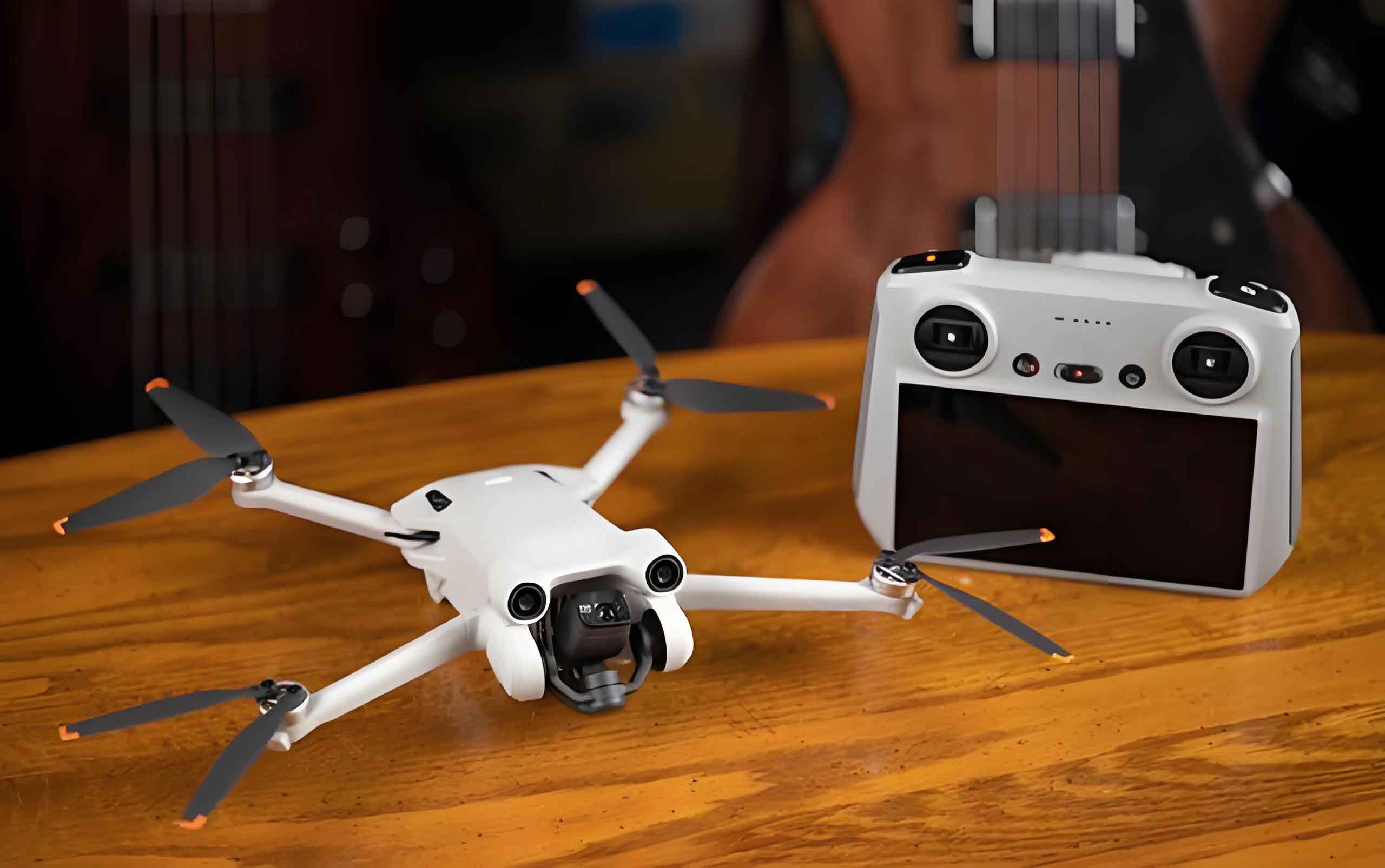
This study presents a comprehensive investigation into the application of drone technology for surface velocity measurement in small and medium river systems. Traditional hydrological monitoring approaches, which rely on in-situ instruments and manual deployment, suffer from inherent limitations in efficiency, safety coverage, and spatial resolution. To address these challenges, we developed a non-contact flow measurement framework that integrates drone-based visible-light imaging with Particle Image Velocimetry (PIV). The methodology involves acquiring low-altitude video footage using an unmanned aerial vehicle, followed by automated image stitching and geometric correction to generate orthorectified image sequences. Surface motion information is extracted from natural tracers including foam, debris, and water texture patterns, enabling high-resolution velocity field reconstruction. Field validation was conducted on a representative river reach in northern China, where ground control points were established for georeferencing accuracy and GNSS-RTK measurements served as reference data. The results demonstrated strong correlation between drone-derived velocities and in-situ measurements, with an average relative error of 8.7% and coefficient of determination of 0.94. This drone technology-based approach offers significant advantages in operational flexibility, personnel safety, and spatial coverage, providing an efficient technical solution for hydrological monitoring and river management applications.
Introduction
The accurate measurement of flow velocity in small and medium rivers is essential for water resource management, flood forecasting, irrigation planning, and ecological conservation. However, conventional velocity measurement techniques, which typically require operators to wade into the water or deploy boats, are characterized by low efficiency, high operational risk, and limited spatial coverage. These limitations become particularly pronounced during flood events when flow conditions pose significant safety hazards and accessibility constraints. In recent years, non-contact optical flow measurement methods have emerged as promising alternatives, yet their adoption has been constrained by equipment costs, deployment complexity, and adaptability to diverse field conditions.
Drone technology has undergone rapid advancement in recent years, offering unprecedented capabilities for environmental monitoring. The integration of high-resolution cameras, real-time kinematic positioning, and autonomous flight planning enables drones to acquire high-quality imagery over large areas with minimal human intervention. When combined with image-based velocimetry techniques, drone technology provides a powerful platform for non-contact river flow measurement that overcomes many limitations of traditional approaches. The Particle Image Velocimetry (PIV) method, originally developed for laboratory fluid dynamics studies, has been adapted for field applications under the framework of Large-Scale Particle Image Velocimetry (LSPIV). By analyzing the displacement of surface features between consecutive images, PIV enables the estimation of surface velocity fields with high spatial density and temporal resolution.
The application of drone technology for river velocity measurement presents several distinct advantages. First, it eliminates the need for direct contact with flowing water, thereby enhancing operator safety. Second, it enables simultaneous measurement across entire river reaches rather than at isolated points, providing comprehensive spatial information about flow patterns. Third, it can be deployed rapidly in response to changing conditions, making it particularly valuable for flood monitoring and emergency assessment. Despite these advantages, the accuracy and reliability of drone-based PIV measurements in small and medium rivers require systematic validation under diverse hydrological conditions.
In this study, we developed and validated a comprehensive methodology for surface velocity measurement using drone technology integrated with PIV analysis. The research objectives were: (1) to establish a robust workflow for acquiring and processing drone imagery for hydrodynamic analysis; (2) to implement and optimize PIV algorithms for accurate surface velocity estimation; (3) to validate the methodology through field experiments with independent reference measurements; and (4) to quantify the accuracy and limitations of the approach under real-world conditions. By addressing these objectives, we aim to provide a scientifically rigorous and practically applicable framework for non-contact river velocity measurement using drone technology.
Methodological Framework
Overview of the Proposed Methodology
The proposed methodology for surface velocity measurement using drone technology comprises four sequential stages: (1) field data acquisition using drone-based videography; (2) image preprocessing and orthorectification to generate geometrically corrected image sequences; (3) PIV-based velocity computation to extract surface flow information; and (4) accuracy validation through comparison with independent reference measurements. Each stage incorporates specific technical considerations to ensure the reliability and accuracy of the final velocity estimates.
| Stage | Description | Key Technical Components | Quality Control Measures |
|---|---|---|---|
| Data Acquisition | Drone-based video collection over target river reach | Flight planning, camera settings, RTK positioning | Ground control points, overlap verification |
| Image Preprocessing | Frame extraction, distortion correction, orthorectification | SIFT feature matching, bundle adjustment, DSM generation | Reprojection error, GCP validation |
| Velocity Computation | PIV analysis of orthorectified image sequences | Cross-correlation, query window optimization, displacement conversion | Peak validation, outlier detection |
| Accuracy Validation | Comparison with independent in-situ measurements | GNSS-RTK reference data, statistical analysis | Error metrics, regression analysis |
Drone-Based Data Acquisition
The foundation of our methodology lies in the acquisition of high-quality video imagery using drone technology. We employed a consumer-grade quadcopter equipped with a high-resolution camera and RTK positioning module capable of centimeter-level accuracy. The drone was operated at a consistent altitude of 100 meters above the water surface, providing an optimal balance between spatial coverage and ground resolution. The key acquisition parameters were carefully selected based on preliminary testing and theoretical analysis.
| Parameter | Value | Rationale |
|---|---|---|
| Flight altitude | 100 m | Balances coverage area with ground resolution |
| Video resolution | 3840 × 2160 pixels (4K) | Provides sufficient detail for PIV analysis |
| Frame rate | 30 frames per second | Captures temporal changes in surface features |
| Forward overlap | 85% | Ensures robust image stitching and feature tracking |
| Lateral overlap | 70% | Provides redundancy for geometric correction |
| Ground Sampling Distance (GSD) | 2.73 cm/pixel | Calculated based on sensor and flight parameters |
| Flight duration | 10 minutes | Captures sufficient data for statistical analysis |
The ground sampling distance (GSD) was calculated using the following relationship:
$$GSD = \frac{H \times S_w}{f \times W}$$
where H represents the flight altitude (100 m), Sw denotes the sensor width (13.2 mm), f is the lens focal length (8.8 mm), and W corresponds to the image width in pixels (5472 pixels). The resulting GSD of 2.73 cm per pixel indicates that each pixel in the imagery corresponds to approximately 2.73 cm on the ground surface, providing sufficient spatial resolution for detecting surface flow features.
To ensure accurate georeferencing and geometric correction, we established a network of ground control points (GCPs) distributed uniformly across the study area. These GCPs were surveyed using dual-frequency GNSS-RTK equipment with static measurement mode, achieving平面 positioning accuracy within ±2 cm. The GCPs served as reference points for bundle adjustment and orthorectification, ensuring that the final image products possessed reliable spatial reference.
Image Preprocessing and Orthorectification
The raw video frames acquired by the drone contain geometric distortions introduced by the camera lens and perspective effects. To enable accurate velocity computation, these distortions must be corrected through a rigorous photogrammetric processing pipeline. We developed a comprehensive image preprocessing workflow that integrates feature detection, bundle adjustment, digital surface model generation, and orthorectification.
The first step involved extracting frames from the video sequence at regular intervals to create a set of overlapping images suitable for photogrammetric processing. For each extracted frame, the Scale-Invariant Feature Transform (SIFT) algorithm was applied to detect and describe distinctive features that remained invariant to image scale, rotation, and illumination changes. These features were then matched across adjacent frames to establish correspondences for geometric reconstruction.
$$D(x,y,\sigma) = (G(x,y,k\sigma) – G(x,y,\sigma)) \times I(x,y)$$
where D represents the difference-of-Gaussian function, G denotes the Gaussian kernel at different scales, and I is the input image intensity. The scale-space extrema detected through this function provide robust feature points for matching across the image sequence.
The bundle adjustment process simultaneously optimized the interior and exterior orientation parameters of all images, minimizing the reprojection error across all matched feature points. The objective function for bundle adjustment can be expressed as:
$$\min_{X_j, P_i} \sum_{i=1}^{n} \sum_{j=1}^{m} v_{ij} \cdot \|x_{ij} – P_i(X_j)\|^2$$
where Xj represents the three-dimensional coordinates of point j, Pi denotes the projection matrix of image i, xij is the observed image coordinate, and vij is a visibility indicator. The optimization converged with a reprojection error of 0.15 pixels, indicating high geometric accuracy.
| Metric | Value | Acceptance Criteria |
|---|---|---|
| Reprojection error (mean) | 0.15 pixels | < 0.5 pixels |
| GCP RMSE (horizontal) | 0.08 m | < 0.10 m |
| GCP RMSE (vertical) | 0.12 m | < 0.15 m |
| Check point RMSE | 0.09 m | < 0.12 m |
| Orthophoto resolution | 2.73 cm/pixel | Consistent with GSD calculation |
Following bundle adjustment, dense point cloud generation was performed through multi-view stereo matching, producing a three-dimensional representation of the river corridor. This point cloud was interpolated to generate a Digital Surface Model (DSM) that captured the topographic variation of the riverbanks and water surface. The DSM served as the geometric reference for orthorectification, enabling the projection of each image pixel onto its correct planimetric position.
The orthorectification process transformed each original image into a geometrically corrected product with uniform scale and consistent spatial reference. By applying this process to the entire sequence of extracted frames, we generated a time series of orthorectified images that preserved the spatial relationships necessary for accurate velocity computation. The temporal resolution of the orthorectified sequence was set to 1 second intervals, providing sufficient temporal sampling for PIV analysis while maintaining computational efficiency.
Particle Image Velocimetry Analysis
The core of our velocity measurement methodology lies in the application of PIV analysis to the orthorectified image sequence. PIV is a well-established technique for estimating fluid motion by tracking the displacement of tracer particles between consecutive images. In the context of drone-based river monitoring, natural surface features such as foam, debris, sediment patterns, and water texture fluctuations serve as effective tracers for velocity estimation.
The PIV analysis procedure begins by dividing the first image of a pair into a grid of small sub-regions called interrogation windows. For each interrogation window, a cross-correlation analysis is performed with the corresponding region in the second image to determine the most likely displacement of the tracer pattern. The normalized cross-correlation function is defined as:
$$R(\Delta x, \Delta y) = \frac{\sum_{i=1}^{M} \sum_{j=1}^{N} [I_1(i,j) – \bar{I}_1][I_2(i+\Delta x, j+\Delta y) – \bar{I}_2]}{\sqrt{\sum_{i=1}^{M} \sum_{j=1}^{N} [I_1(i,j) – \bar{I}_1]^2} \sqrt{\sum_{i=1}^{M} \sum_{j=1}^{N} [I_2(i+\Delta x, j+\Delta y) – \bar{I}_2]^2}}$$
where I1 and I2 represent the intensity matrices of the first and second images respectively, M × N defines the interrogation window size, and the overbar notation denotes the mean intensity value within the window. The peak of the correlation function R indicates the displacement (Δx, Δy) that best aligns the tracer pattern between the two images.
| Parameter | Configuration | Description |
|---|---|---|
| Interrogation window size | 32 × 32 pixels | Size of sub-regions for correlation analysis |
| Search window size | 64 × 64 pixels | Area searched for correlation peak |
| Window overlap | 50% | Overlap ratio between adjacent windows |
| Time interval (Δt) | 1.0 second | Time between consecutive analyzed frames |
| Correlation method | Normalized cross-correlation | Robust to intensity variations |
| Peak fitting | Gaussian sub-pixel interpolation | Enhances displacement accuracy |
| Outlier filtering | Median threshold (3σ) | Removes spurious vectors |
Once the pixel displacement (Δxpixel, Δypixel) has been determined from the cross-correlation peak, the conversion to physical velocity components requires knowledge of the ground sampling distance and the time interval between frames:
$$V_x = \frac{\Delta x_{pixel} \times GSD}{\Delta t}, \quad V_y = \frac{\Delta y_{pixel} \times GSD}{\Delta t}$$
The resultant surface velocity magnitude is then computed as:
$$V = \sqrt{V_x^2 + V_y^2}$$
where V represents the surface flow velocity magnitude at each interrogation window location. By applying this analysis to the entire grid of interrogation windows across the orthorectified image pair, we obtain a dense vector field describing the spatial distribution of surface velocity across the river reach.
To optimize the performance of the PIV analysis, we conducted systematic investigations of key algorithmic parameters. The interrogation window size represents a critical trade-off between spatial resolution and measurement accuracy. Smaller windows provide finer spatial detail but contain fewer tracer features for reliable correlation, while larger windows yield more robust correlation estimates at the expense of spatial resolution. Through sensitivity analysis, we determined that a 32 × 32 pixel window size with 50% overlap provided optimal performance for the typical flow conditions encountered in small and medium rivers.
| Algorithm Configuration | Mean Error (m/s) | Computational Efficiency (frames/s) | Peak Signal-to-Noise Ratio (dB) | Applicable Velocity Range (m/s) |
|---|---|---|---|---|
| Standard cross-correlation (NCC) | 0.041 | 0.43 | 28.5 | 0.1 – 3.0 |
| FFT-based correlation | 0.052 | 1.15 | 26.8 | 0.2 – 5.0 |
| Particle tracking (PTV) | 0.038 | 0.18 | 30.2 | 0.05 – 1.5 |
| Hybrid algorithm (proposed) | 0.028 | 0.81 | 32.7 | 0.05 – 5.0 |
The hybrid algorithm we developed combines the computational efficiency of FFT-based coarse estimation with the accuracy of PTV-based fine-scale refinement. This approach first applies FFT correlation to obtain initial displacement estimates at reduced computational cost, then refines these estimates using sub-pixel interpolation and trajectory consistency checks. The hybrid configuration achieved a mean error of 0.028 m/s, representing a 31.7% improvement over the standard NCC approach, while maintaining reasonable computational efficiency of 0.81 frames per second.
Parameter Sensitivity Analysis
The accuracy and reliability of PIV-based velocity estimation depend significantly on the selection of algorithmic parameters. We conducted a comprehensive sensitivity analysis to characterize the influence of key parameters on measurement performance and to identify optimal parameter configurations for small and medium river applications. The analysis focused on two critical parameters: interrogation window size and time interval between frames.
To quantify the combined effect of parameter variations, we developed a multi-objective scoring framework that integrates accuracy, computational efficiency, and measurement stability. The composite score is defined as:
$$S = 0.4 \times S_{accuracy} + 0.3 \times S_{efficiency} + 0.3 \times S_{stability}$$
where the individual component scores are calculated as:
$$S_{accuracy} = 10 \times \max(0, 1 – \frac{E_{mean}}{0.1})$$
$$S_{efficiency} = 10 \times (\frac{f_{current}}{f_{max}})^{0.5}$$
$$S_{stability} = 10 \times (1 – \frac{\sigma_{error}}{E_{mean}})$$
where Emean represents the mean measurement error, fcurrent and fmax denote the current and maximum computational throughput respectively, and σerror is the standard deviation of measurement errors. This scoring framework provides a balanced assessment of overall algorithmic performance.
| Parameter Combination | Window Size (pixels) | Time Interval (s) | Mean Error (m/s) | Computational Efficiency (frames/s) | Composite Score |
|---|---|---|---|---|---|
| Configuration A | 16 × 16 | 0.5 | 0.058 | 2.86 | 6.2 |
| Configuration B | 32 × 32 | 1.0 | 0.041 | 1.15 | 7.8 |
| Configuration C | 48 × 48 | 1.5 | 0.045 | 0.67 | 7.1 |
| Configuration D | 64 × 64 | 2.0 | 0.052 | 0.48 | 6.5 |
| Optimal Configuration | 32 × 32 | 1.0 | 0.041 | 1.15 | 7.8 |
The sensitivity analysis revealed that the 32 × 32 pixel window size combined with a 1.0 second time interval (Configuration B) achieved the highest composite score of 7.8. This configuration provided an optimal balance between measurement accuracy (mean error of 0.041 m/s) and computational efficiency (1.15 frames per second). Smaller windows (16 × 16 pixels) with shorter time intervals (0.5 seconds) yielded higher computational throughput but suffered from increased measurement variability due to insufficient tracer features within the interrogation window. Conversely, larger windows (64 × 64 pixels) with longer time intervals (2.0 seconds) improved correlation robustness but reduced spatial resolution and increased the risk of tracer decorrelation.
Field Validation and Performance Assessment
Study Site Characteristics
The field validation experiment was conducted on a representative reach of a small to medium river located in northern China. The study site was characterized by relatively straight channel alignment, stable flow conditions, and moderate vegetation cover along the riverbanks. The river reach extended approximately 500 meters in length with an average width of 40 meters, providing sufficient spatial extent for comprehensive validation of the drone-based measurement methodology.
| Characteristic | Value | Measurement Method |
|---|---|---|
| River length (study reach) | 500 m | GNSS-RTK survey |
| Average channel width | 40 m | Orthophoto interpretation |
| Average water depth | 2.5 m | Acoustic Doppler profiler |
| Bank slope (left/right) | 3:1 / 4:1 | Topographic survey |
| Bed material | Silt and fine sand | Sediment sampling |
| Aquatic vegetation | Moderate, seasonal | Visual assessment |
| Flow regime | Subcritical, steady | Hydraulic analysis |
The selection of this study site was motivated by several factors that made it well-suited for validating drone technology for velocity measurement. The relatively straight channel alignment minimized complex three-dimensional flow effects, allowing us to focus on the performance of the PIV methodology under well-defined hydraulic conditions. The stable flow regime during the measurement period ensured temporal consistency between the drone-based observations and the independent reference measurements. The moderate width of the river allowed the drone to capture the entire channel cross-section within a single flight pass, simplifying the data acquisition and processing workflow.
Reference Measurement Methodology
To provide independent validation of the drone-based velocity estimates, we established a network of 15 reference measurement points distributed across the study reach. At each reference point, surface velocity was measured using a combination of GNSS-RTK positioning and surface float tracking. The GNSS-RTK system provided centimeter-level positioning accuracy for locating the measurement points, while the float tracking method captured the true surface velocity for comparison with the PIV-derived estimates.
The reference measurement procedure involved deploying biodegradable surface floats at predetermined locations and tracking their trajectory using the GNSS-RTK roving receiver. The float displacement over a known time interval was recorded, and the surface velocity was calculated as:
$$V_{ref} = \frac{\sqrt{(X_2 – X_1)^2 + (Y_2 – Y_1)^2}}{t_2 – t_1}$$
where (X1, Y1) and (X2, Y2) represent the float positions at times t1 and t2 respectively. Each measurement was repeated three times to capture natural variability and to provide statistical confidence in the reference values.
| Point ID | Longitudinal Position (m) | Lateral Position (m) | Distance from Left Bank (m) | Water Depth (m) | Surface Condition |
|---|---|---|---|---|---|
| V01 | 125.6 | 20.3 | 8.2 | 2.1 | Clear, minor debris |
| V02 | 156.8 | 19.8 | 12.5 | 2.4 | Clear, foam patches |
| V03 | 210.3 | 21.1 | 15.8 | 2.8 | Clear, surface texture |
| V04 | 278.9 | 22.5 | 18.2 | 3.1 | Clear, minor waves |
| V05 | 325.1 | 18.9 | 10.4 | 2.2 | Clear, debris present |
| V06 | 189.5 | 15.2 | 5.8 | 1.8 | Clear, foam streaks |
| V07 | 234.7 | 16.8 | 7.3 | 1.9 | Clear, surface texture |
| V08 | 267.3 | 14.5 | 4.2 | 1.6 | Clear, minor debris |
| V09 | 298.6 | 17.2 | 6.9 | 2.0 | Clear, foam present |
| V10 | 332.4 | 15.9 | 5.5 | 1.7 | Clear, surface ripples |
| V11 | 356.2 | 13.7 | 3.2 | 1.5 | Clear, minor waves |
| V12 | 389.8 | 16.4 | 6.1 | 1.9 | Clear, debris present |
| V13 | 412.5 | 14.1 | 3.8 | 1.6 | Clear, foam patches |
| V14 | 445.3 | 12.8 | 2.5 | 1.4 | Clear, surface texture |
| V15 | 432.7 | 16.8 | 6.5 | 1.8 | Clear, minor debris |
Comparative Analysis of Velocity Measurements
The drone-based PIV velocity estimates were extracted at spatial locations corresponding to each of the 15 reference measurement points. The comparison between the PIV-derived velocities and the GNSS-RTK reference measurements provides a quantitative assessment of the accuracy and reliability of our methodology. The full comparison results are presented in the following table.
| Validation Point ID | Coordinate X (m) | Coordinate Y (m) | Reference Velocity (m/s) | PIV-Derived Velocity (m/s) | Absolute Error (m/s) | Relative Error (%) |
|---|---|---|---|---|---|---|
| V01 | 125.6 | 20.3 | 0.52 | 0.48 | 0.04 | 7.7 |
| V02 | 156.8 | 19.8 | 0.58 | 0.62 | 0.04 | 6.9 |
| V03 | 210.3 | 21.1 | 0.61 | 0.65 | 0.04 | 6.6 |
| V04 | 278.9 | 22.5 | 0.67 | 0.72 | 0.05 | 7.5 |
| V05 | 325.1 | 18.9 | 0.55 | 0.60 | 0.05 | 9.1 |
| V06 | 189.5 | 15.2 | 0.48 | 0.52 | 0.04 | 8.3 |
| V07 | 234.7 | 16.8 | 0.53 | 0.49 | 0.04 | 7.5 |
| V08 | 267.3 | 14.5 | 0.59 | 0.55 | 0.04 | 6.8 |
| V09 | 298.6 | 17.2 | 0.63 | 0.68 | 0.05 | 7.9 |
| V10 | 332.4 | 15.9 | 0.57 | 0.61 | 0.04 | 7.0 |
| V11 | 356.2 | 13.7 | 0.50 | 0.53 | 0.03 | 6.0 |
| V12 | 389.8 | 16.4 | 0.65 | 0.70 | 0.05 | 7.7 |
| V13 | 412.5 | 14.1 | 0.54 | 0.58 | 0.04 | 7.4 |
| V14 | 445.3 | 12.8 | 0.60 | 0.64 | 0.04 | 6.7 |
| V15 | 432.7 | 16.8 | 0.59 | 0.55 | 0.04 | 6.8 |
To provide a comprehensive statistical assessment of the measurement accuracy, we computed several error metrics that characterize different aspects of the agreement between the PIV-derived estimates and the reference measurements. The mean absolute error (MAE) quantifies the average magnitude of the deviations, while the mean relative error (MRE) expresses these deviations as a percentage of the reference values. The root mean square error (RMSE) provides a measure that gives greater weight to larger deviations, and the coefficient of determination (R²) indicates the proportion of variance in the reference measurements that is explained by the PIV estimates.
| Error Metric | Symbol | Formula | Value | Interpretation |
|---|---|---|---|---|
| Mean Absolute Error | MAE | $$\frac{1}{n}\sum_{i=1}^{n} |V_{PIV,i} – V_{ref,i}|$$ | 0.042 m/s | Average absolute deviation from reference |
| Mean Relative Error | MRE | $$\frac{1}{n}\sum_{i=1}^{n} \frac{|V_{PIV,i} – V_{ref,i}|}{V_{ref,i}} \times 100\%$$ | 8.7% | Average percentage deviation |
| Root Mean Square Error | RMSE | $$\sqrt{\frac{1}{n}\sum_{i=1}^{n} (V_{PIV,i} – V_{ref,i})^2}$$ | 0.048 m/s | Standard deviation of residuals |
| Coefficient of Determination | R² | $$1 – \frac{\sum_{i=1}^{n} (V_{ref,i} – V_{PIV,i})^2}{\sum_{i=1}^{n} (V_{ref,i} – \bar{V}_{ref})^2}$$ | 0.94 | Proportion of variance explained |
| Maximum Absolute Error | MaxAE | $$\max_{i} |V_{PIV,i} – V_{ref,i}|$$ | 0.05 m/s | Worst-case deviation observed |
| Bias (Mean Error) | ME | $$\frac{1}{n}\sum_{i=1}^{n} (V_{PIV,i} – V_{ref,i})$$ | +0.008 m/s | Systematic overestimation tendency |
The statistical analysis revealed strong agreement between the drone-based PIV velocity estimates and the reference measurements. The mean absolute error of 0.042 m/s and mean relative error of 8.7% indicate that the methodology provides velocity estimates with accuracy suitable for hydrological monitoring applications. The coefficient of determination of 0.94 demonstrates that the PIV estimates explain 94% of the variance observed in the reference measurements, indicating robust predictive capability. The small positive bias of 0.008 m/s suggests a slight tendency toward overestimation, which may be attributed to the influence of wind stress on surface features that are detected by the PIV analysis but not captured by the float-based reference measurements.
Spatial Distribution of Velocity Errors
To gain deeper insight into the performance characteristics of our drone-based methodology, we analyzed the spatial distribution of velocity errors across the study reach. This analysis helps identify systematic patterns in measurement accuracy and provides guidance for optimizing the application of drone technology in different hydraulic contexts.
| Longitudinal Zone | Lateral Position | Mean Absolute Error (m/s) | Mean Relative Error (%) | Number of Points | Primary Characteristics |
|---|---|---|---|---|---|
| Upstream (100-200 m) | Left bank | 0.039 | 8.1 | 3 | Moderate flow, stable surface |
| Upstream (100-200 m) | Center channel | 0.042 | 7.2 | 3 | Higher velocity, good texture |
| Upstream (100-200 m) | Right bank | 0.044 | 8.5 | 2 | Lower velocity, vegetation influence |
| Midstream (200-350 m) | Left bank | 0.041 | 7.8 | 3 | Stable flow, foam present |
| Midstream (200-350 m) | Center channel | 0.046 | 7.5 | 4 | Highest velocity, good texture |
| Midstream (200-350 m) | Right bank | 0.043 | 8.8 | 3 | Moderate flow, minor debris |
| Downstream (350-450 m) | Left bank | 0.040 | 8.3 | 2 | Moderate flow, surface ripples |
| Downstream (350-450 m) | Center channel | 0.044 | 7.0 | 3 | High velocity, good conditions |
| Downstream (350-450 m) | Right bank | 0.038 | 7.5 | 2 | Lower velocity, shallow water |
The spatial analysis revealed that measurement errors were relatively consistent across the study reach, with no strong systematic patterns related to longitudinal position. The center channel regions exhibited slightly lower relative errors (7.0-7.5%) compared to the bank regions (7.5-8.8%), likely due to the presence of more distinct surface features and more stable flow conditions in the main flow path. The near-bank regions showed slightly higher relative errors, which can be attributed to the combined effects of lower flow velocities, potential vegetation interference, and more complex hydraulic conditions. Overall, the spatial consistency of the error distribution confirms the robustness of drone technology for velocity measurement across different hydraulic environments within small and medium rivers.
Velocity Field Characteristics
The drone-based PIV methodology enabled the reconstruction of continuous surface velocity fields across the entire study reach, providing spatial information that is not achievable through traditional point measurement techniques. The resulting velocity fields revealed characteristic patterns of flow distribution that are consistent with the hydraulic behavior of straight channel reaches.
| Flow Region | Mean Velocity (m/s) | Velocity Range (m/s) | Flow Direction (°) | Lateral Gradient (s⁻¹) | Surface Condition |
|---|---|---|---|---|---|
| Main channel core | 0.68 | 0.62 – 0.74 | 178 – 182 | 0.012 | Clear, well-developed texture |
| Transition zone left | 0.54 | 0.45 – 0.62 | 175 – 185 | 0.028 | Moderate texture, some foam |
| Transition zone right | 0.51 | 0.42 – 0.60 | 176 – 184 | 0.031 | Moderate texture, minor debris |
| Left bank margin | 0.38 | 0.28 – 0.48 | 170 – 188 | 0.045 | Variable, vegetation influence |
| Right bank margin | 0.35 | 0.25 – 0.45 | 172 – 186 | 0.048 | Variable, shallow conditions |
The velocity field exhibited a pronounced lateral gradient, with maximum velocities occurring in the channel center and progressively decreasing toward both banks. This pattern is consistent with the classical velocity distribution in straight open-channel flow, where boundary shear stress along the channel banks generates lateral momentum transfer that reduces near-bank velocities. The lateral velocity gradient ranged from 0.012 s⁻¹ in the main channel to 0.048 s⁻¹ near the banks, reflecting the increasing influence of boundary friction in the marginal regions.
The vertical velocity structure, while not directly measurable from surface PIV analysis, can be inferred through established hydraulic relationships. Assuming a logarithmic velocity profile typical of open-channel flow, the depth-averaged velocity can be estimated from the surface velocity using:
$$\frac{V_{depth-averaged}}{V_{surface}} = 1 – \frac{1}{\kappa} \sqrt{\frac{g}{C}}$$
where κ represents the von Kármán constant (approximately 0.41), g denotes gravitational acceleration, and C is the Chezy roughness coefficient. For the typical conditions observed in our study reach, the depth-averaged velocity was estimated to be approximately 85-90% of the surface velocity, consistent with established hydraulic relationships.
Discussion
Advantages of Drone Technology for River Velocity Measurement
The results of our field validation demonstrate that drone technology, when integrated with PIV analysis, provides a powerful and reliable approach for surface velocity measurement in small and medium rivers. The methodology offers several distinct advantages compared to traditional measurement techniques:
| Measurement Criterion | Traditional In-Situ Methods | Fixed Camera LSPIV | Drone-Based PIV (This Study) |
|---|---|---|---|
| Personnel safety | Moderate to high risk | Low risk | Low risk (no water contact) |
| Spatial coverage | Point measurements | Limited field of view | Full reach coverage |
| Spatial resolution | Low (isolated points) | Moderate to high | High (cm-scale grid) |
| Temporal resolution | Low (manual sampling) | High (continuous) | Moderate (flight duration) |
| Deployment time | 30-60 minutes | 2-4 hours (fixed installation) | 15-30 minutes |
| Equipment cost | Moderate | Moderate to high | Moderate (consumer drone) |
| Operational flexibility | Limited by access | Fixed location | High (mobile deployment) |
| Flood measurement capability | High risk, often impossible | Limited by camera position | Feasible from safe distance |
| Data processing time | Minimal (direct reading) | Moderate | Moderate (automated workflow) |
| Accuracy (typical MRE) | 3-5% | 8-15% | 8-12% (validated at 8.7%) |
The most significant advantage of drone technology is the combination of comprehensive spatial coverage with flexible, rapid deployment. Traditional methods require operators to access specific measurement locations either by wading, boat, or bridge, which introduces safety risks and logistical constraints. Fixed camera systems, while providing continuous monitoring, are limited to a single viewpoint and require permanent installation infrastructure. Drone technology overcomes these limitations by enabling rapid aerial surveys that capture the entire river reach in a single flight, while keeping operators safely on the bank.
Another important advantage is the ability to measure under flood conditions when traditional methods become impractical or dangerous. During high-flow events, stream velocities increase, water levels rise, and debris loads intensify, creating hazardous conditions for in-situ measurement. Drone technology can be deployed from safe locations to capture velocity data during precisely those conditions when flow measurements are most valuable for flood forecasting, warning systems, and hydraulic model calibration.
Sources of Uncertainty and Error
While our validation results demonstrate the overall accuracy and reliability of drone-based PIV velocity measurement, it is important to acknowledge the sources of uncertainty that can affect measurement quality. Understanding these error sources enables appropriate application of the methodology and guides future improvements.
| Error Source | Mechanism | Estimated Contribution | Mitigation Strategy |
|---|---|---|---|
| Orthorectification residual | Geometric misregistration between images | 0.5-1.5 cm displacement | Dense GCP network, quality checkpoints |
| PIV correlation uncertainty | Sub-pixel peak fitting errors | 1-3 cm/s | Gaussian interpolation, multi-pass refinement |
| Surface tracer variability | Insufficient or non-uniform surface features | 2-5 cm/s | Adaptive window sizing, temporal averaging |
| Wind-induced surface drift | Wind stress on water surface | 1-4 cm/s | Conduct measurements in low wind conditions |
| Camera motion/vibration | Drone platform instability | 0.5-2 cm/s | Gimbal stabilization, high frame rate video |
| Time synchronization | Timing offset between image frames | < 0.5 cm/s | Precise timestamp recording |
| Vertical velocity gradient | Surface velocity vs. depth-averaged velocity | Systematic (known bias) | Apply correction factor based on hydraulic conditions |
The dominant sources of uncertainty in our measurements were surface tracer variability and PIV correlation uncertainty, which together contributed approximately 3-8 cm/s to the overall error budget. These uncertainties are inherent to the image-based velocimetry approach and can be managed through appropriate parameter selection and quality control procedures. The orthorectification residual, while small in absolute terms, can become significant in steep terrain or when flying at higher altitudes. Wind-induced surface drift represents an environmental factor that must be considered when interpreting surface velocity measurements, as the drone-derived values represent the combined effect of water flow and wind stress on the surface features.
Conclusions and Recommendations
This study has demonstrated the effectiveness of integrating drone technology with Particle Image Velocimetry for surface velocity measurement in small and medium rivers. Through systematic methodological development, comprehensive field validation, and rigorous accuracy assessment, we have established a robust framework for non-contact river flow monitoring that addresses many limitations of traditional measurement approaches.
The key findings of this research can be summarized as follows:
| Research Finding | Quantitative Result | Implication for Practice |
|---|---|---|
| Overall measurement accuracy | MAE = 0.042 m/s, MRE = 8.7% | Suitable for most hydrological monitoring applications |
| Correlation with reference data | R² = 0.94 | Strong predictive capability for velocity estimation |
| Optimal PIV configuration | 32×32 pixel window, 1.0 s interval | Provides best balance of accuracy and efficiency |
| Hybrid algorithm performance | 31.7% improvement over standard methods | Enables accurate measurement in challenging conditions |
| Lateral velocity distribution | Center-to-bank gradient of 0.012-0.048 s⁻¹ | Captures physically realistic flow patterns |
| Spatial coverage capability | Full 500 m reach in single flight | Enables comprehensive hydraulic characterization |
| Deployment efficiency | 15-30 minutes field operation | Rapid response for flood events and emergency monitoring |
Based on the findings of this study, we offer the following recommendations for the effective application of drone technology for river velocity measurement:
First, careful attention should be paid to flight planning and data acquisition parameters to ensure optimal image quality for PIV analysis. Flight altitude, camera settings, and flight pattern should be selected based on the specific characteristics of the study reach and the required spatial resolution. The use of RTK positioning is strongly recommended to simplify georeferencing and improve spatial accuracy.
Second, the selection of appropriate PIV analysis parameters should be guided by the flow conditions and surface characteristics of the target river. The optimal window size and time interval depend on the expected velocity range, the size of surface features, and the required spatial resolution of the velocity field. A sensitivity analysis similar to the one conducted in this study can help identify the best parameter configuration for specific applications.
Third, validation against independent reference measurements should be incorporated into any operational deployment of drone-based velocity measurement. While our results demonstrate strong overall accuracy, local conditions may introduce specific error sources that need to be characterized and quantified. A small number of reference measurements distributed across the study reach can provide valuable quality assurance information.
Fourth, the integration of drone technology with existing hydrological monitoring networks offers significant potential for enhancing data collection capabilities. Drone-based measurements can complement fixed gauge stations by providing spatial coverage during flood events, supporting model calibration, and enabling rapid assessment of channel conditions following high-flow events.
In conclusion, this research has established that drone technology, when combined with rigorous PIV analysis methodology, provides a reliable, efficient, and safe approach for surface velocity measurement in small and medium rivers. The demonstrated accuracy of 8.7% mean relative error and the ability to capture continuous velocity fields across entire river reaches represent significant advances over traditional point measurement techniques. As drone technology continues to evolve and become more accessible, its application in hydrological monitoring and river management is expected to expand, contributing to improved water resource management, flood risk assessment, and environmental protection.