
We investigate the problem of distributed fixed-time formation tracking control for a swarm of fixed-wing UAVs. The goal is to enable the swarm to achieve and maintain a desired formation configuration within a prescribed fixed time, regardless of initial conditions, while accounting for actuator unmodeled dynamics and uncertainties. Our approach is based on a novel fixed-time terminal sliding mode that guarantees convergence time independent of initial states. We design a distributed cooperative controller that ensures robust tracking under external disturbances and prove fixed-time stability via Lyapunov theory. Numerical simulations validate the effectiveness of our controller.
1. Introduction
In recent years, fixed-wing UAV technology has advanced rapidly, yet single UAVs suffer from high cost, long development cycles, and limited fault tolerance. Swarm operations using multiple low-cost fixed-wing UAVs offer improved robustness and scalability, making them attractive for both civilian and military applications. Formation tracking control is a key challenge in UAV swarms, where problems include actuator uncertainties, external disturbances, and the need for finite-time or fixed-time convergence. While finite-time control ensures convergence within a bounded time dependent on initial conditions, fixed-time control provides a convergence bound independent of initial states. This property is crucial for time-critical missions such as obstacle avoidance formation reconfiguration.
Existing works have addressed finite-time formation control for fixed-wing UAV swarms, but few have tackled the fixed-time problem with actuator dynamics and uncertainties. We extend the fixed-time terminal sliding mode approach to a fully nonlinear 3-DOF model of fixed-wing UAVs, designing a distributed controller that ensures fixed-time formation tracking even under unknown bounded disturbances.
2. Problem Formulation
2.1 Fixed-Wing UAV Dynamics
We consider a swarm of \( N \) fixed-wing UAVs. The 3-DOF point-mass model in the Earth-fixed frame (North-East-Up) is:
$$
\begin{aligned}
\dot{x}_i &= V_i \cos\gamma_i \cos\chi_i, \\
\dot{y}_i &= V_i \cos\gamma_i \sin\chi_i, \\
\dot{z}_i &= V_i \sin\gamma_i, \\
\dot{V}_i &= (V_{c_i} – V_i)/\tau_V, \\
\dot{\chi}_i &= (\chi_{c_i} – \chi_i)/\tau_\chi, \\
\dot{\gamma}_i &= (\gamma_{c_i} – \gamma_i)/\tau_\gamma,
\end{aligned}
$$
where \( i=1,\dots,N \), \( (x_i,y_i,z_i) \) are position coordinates, \( V_i \) is ground speed, \( \gamma_i \) is flight path angle, \( \chi_i \) is heading angle, \( V_{c_i},\chi_{c_i},\gamma_{c_i} \) are control inputs, and \( \tau_V,\tau_\chi,\tau_\gamma \) are time constants.
We rewrite the model in vector form with actuator uncertainties:
$$
\begin{aligned}
\dot{\mathbf{p}}_i &= \mathbf{v}_i, \\
\dot{\mathbf{v}}_i &= \mathbf{u}_i + \mathbf{d}_i,
\end{aligned}
$$
where \( \mathbf{p}_i=[x_i,y_i,z_i]^T \), \( \mathbf{v}_i=[v_{x_i},v_{y_i},v_{z_i}]^T \), \( \mathbf{u}_i=[u_{x_i},u_{y_i},u_{z_i}]^T \) is the control input, and \( \mathbf{d}_i \) represents unmodeled dynamics and uncertainties bounded by \( \|\mathbf{d}_i\|\le d_{\max} \).
The transformation between the physical controls and \( \mathbf{u}_i \) is given by:
$$
\begin{aligned}
V_{c_i} &= \tau_V\big[ (u_{x_i}+d_{x_i})\cos\gamma_i\cos\chi_i + (u_{y_i}+d_{y_i})\cos\gamma_i\sin\chi_i + (u_{z_i}+d_{z_i})\sin\gamma_i\big] + V_i, \\
\chi_{c_i} &= \tau_\chi\frac{-(u_{x_i}+d_{x_i})\sin\chi_i + (u_{y_i}+d_{y_i})\cos\chi_i}{V_i\cos\gamma_i} + \chi_i, \\
\gamma_{c_i} &= \frac{\tau_\gamma}{V_i}\big[ -(u_{x_i}+d_{x_i})\sin\gamma_i\cos\chi_i – (u_{y_i}+d_{y_i})\sin\gamma_i\sin\chi_i + (u_{z_i}+d_{z_i})\cos\gamma_i\big] + \gamma_i.
\end{aligned}
$$
2.2 Communication Topology
We consider an undirected communication graph \( \mathcal{G}=(\mathcal{V},\mathcal{E},\mathcal{A}) \) among the fixed-wing UAVs, where \( \mathcal{V}=\{1,\dots,N\} \), \( \mathcal{E} \) are edges, and \( \mathcal{A}=[a_{ij}] \) is the adjacency matrix (\( a_{ij}=1 \) if UAV \( i \) receives information from UAV \( j \)). We also have a virtual leader with state \( \mathbf{p}_d, \mathbf{v}_d \) satisfying \( \dot{\mathbf{p}}_d=\mathbf{v}_d \), \( \dot{\mathbf{v}}_d=\mathbf{g}_d \). The leader adjacency matrix is \( \mathbf{B}=\mathrm{diag}\{b_1,\dots,b_N\} \) with \( b_i=1 \) if UAV \( i \) can access the leader. Define \( \mathbf{H}=\mathbf{L}+\mathbf{B} \), where \( \mathbf{L} \) is the Laplacian. The overall tracking error for the swarm is:
$$
\mathbf{e}_1 = [(\mathbf{L}+\mathbf{B})\otimes \mathbf{I}_3] \mathbf{e}_p,\quad \mathbf{e}_2 = [(\mathbf{L}+\mathbf{B})\otimes \mathbf{I}_3] \mathbf{e}_v,
$$
where \( \mathbf{e}_p = \mathbf{p}_i – (\mathbf{p}_d+\mathbf{h}_{p_i}) \) and \( \mathbf{e}_v = \mathbf{v}_i – (\mathbf{v}_d+\mathbf{h}_{v_i}) \), with \( \mathbf{h}_{p_i},\mathbf{h}_{v_i} \) being the desired formation offsets.
3. Controller Design
3.1 Fixed-Time Terminal Sliding Mode
We adopt a sliding surface that ensures fixed-time convergence once sliding mode is established. For a scalar variable \( x \), define:
$$
s = \dot{x} + f_s(x),
$$
where
$$
f_s(x)=\begin{cases}
\alpha_1 \mathrm{sig}^{p_1}(x) + \beta_1 \mathrm{sig}^{g_1}(x), & \text{if } \bar{s}=0 \text{ or } (\bar{s}\neq0, |x|>\mu), \\
\alpha_2 x + \beta_2 \mathrm{sig}^{2}(x), & \text{if } \bar{s}\neq0, |x|\le\mu,
\end{cases}
$$
with \( \bar{s}=\dot{x}+\alpha_1\mathrm{sig}^{p_1}(x)+\beta_1\mathrm{sig}^{g_1}(x) \), \( \mu>0 \), \( \alpha_1,\beta_1>0 \), \( 0<p_11 \), and parameters \( \alpha_2,\beta_2 \) chosen to ensure continuity. The convergence time satisfies:</p_1
$$
T_{ft} = \frac{1}{\alpha_1(1-p_1)} + \frac{1}{\beta_1(g_1-1)}.
$$
For the fixed-wing UAV formation problem, we define the sliding vector for UAV \( i \) as:
$$
\mathbf{s}_i = \mathbf{e}_{2i} + b_i \mathbf{f}_{si}(\mathbf{e}_{1i}) + \sum_{j=1}^N l_{ij} \mathbf{f}_{sj}(\mathbf{e}_{1j}),
$$
where \( \mathbf{f}_{si} \) applies \( f_s \) elementwise. In stacked form:
$$
\mathbf{s} = \mathbf{H}_1[\mathbf{e}_2 + \mathbf{f}_s(\mathbf{e}_1)],
$$
with \( \mathbf{H}_1 = (\mathbf{L}+\mathbf{B})\otimes \mathbf{I}_3 \).
3.2 Distributed Controller
We propose the following control law for each fixed-wing UAV:
$$
\mathbf{u}_i = -l_1 \mathrm{sig}^{p_2}(\mathbf{s}_i) – l_2 \mathrm{sig}^{g_2}(\mathbf{s}_i) – \boldsymbol{\psi}_i – \dot{\mathbf{f}}_{si}(\mathbf{e}_{1i}),
$$
where \( l_1,l_2>0 \), \( 0<p_21 \), and \( \boldsymbol{\psi}_i \) is a robust term:</p_2
$$
\psi_{im} = \kappa_i \tanh\!\left(\frac{3k_u\kappa_i s_{im}}{\zeta}\right),\quad m=1,2,3,
$$
with \( \kappa_i \ge d_{\max}+\|\mathbf{u}_{di}\| \), \( k_u>0 \), \( \zeta>0 \). The derivative \( \dot{\mathbf{f}}_{si} \) is computed elementwise as:
$$
\dot{f}_{si_m}=\begin{cases}
\alpha_1 p_1 |e_{p_{im}}|^{p_1-1} e_{v_{im}} + \beta_1 g_1 |e_{p_{im}}|^{g_1-1} e_{v_{im}}, & \text{if } \bar{s}_{im}=0 \text{ or } (\bar{s}_{im}\neq0, |e_{p_{im}}|>\mu), \\
\alpha_2 e_{v_{im}} + 2\beta_2 e_{p_{im}} e_{v_{im}}, & \text{if } \bar{s}_{im}\neq0, |e_{p_{im}}|\le\mu.
\end{cases}
$$
The robust term satisfies:
$$
\mathbf{s}_i^T(\mathbf{d}_i – \mathbf{u}_{di}) – \mathbf{s}_i^T\boldsymbol{\psi}_i \le \zeta.
$$
3.3 Stability Analysis
Theorem 1: Consider the fixed-wing UAV swarm (1) with undirected connected communication topology and desired formation offsets \( \mathbf{h}_p,\mathbf{h}_v \). Under control law (14), the sliding surface \( \mathbf{s} \) converges to a small region \( \Omega_1 \) in fixed time \( T_1 \), and the tracking errors \( \mathbf{e}_p, \mathbf{e}_v \) converge to a region \( \Omega_2 \) in fixed time \( T = T_1 + T_2 \), where:
$$
T_1 = \frac{2}{\tau_m(1-p_2)} + \frac{2}{\delta_m(g_2-1)},
$$
$$
\tau_m = l_1\left(\frac{2}{\lambda_{\max}(\mathbf{H}_2)}\right)^{\frac{p_2+1}{2}},\quad
\delta_m = l_2 (3N)^{\frac{1-g_2}{2}} \left(\frac{2}{\lambda_{\max}(\mathbf{H}_2)}\right)^{\frac{g_2+1}{2}},
$$
$$
T_2 = \frac{1}{\alpha_1(1-p_1)} + \frac{1}{\beta_1(g_1-1)}.
$$
Proof sketch: Choose Lyapunov function \( V = \frac12 \mathbf{s}^T\mathbf{H}_2 \mathbf{s} \) with \( \mathbf{H}_2 = \mathbf{H}_1^{-1} \). Its derivative yields:
$$
\dot{V} \le -\tau_m V^{\frac{p_2+1}{2}} – \delta_m V^{\frac{g_2+1}{2}} + N\zeta.
$$
Following Lemma 2 (fixed-time stability from Polyakov), we conclude \( \mathbf{s} \) enters \( \Omega_1 \) within \( T_1 \). Subsequently, the sliding dynamics guarantee that \( \mathbf{e}_1 \) and \( \mathbf{e}_2 \) converge to a residual set around zero within \( T_2 \), independent of initial conditions. The detailed analysis follows [16]. ∎
4. Numerical Simulation
4.1 Simulation Setup
We simulate a swarm of \( N=3 \) fixed-wing UAVs with a virtual leader. The communication graph is fully connected (all UAVs communicate with each other), and UAV 2 receives leader information. Initial conditions and formation offsets are given in Table 1.
| Parameter | Value | Unit |
|---|---|---|
| \( \mathbf{p}_1(0) \) | \( [75.89, -136.09, 55.19]^T \) | m |
| \( \mathbf{p}_2(0) \) | \( [-1.72, 1.54, 60.03]^T \) | m |
| \( \mathbf{p}_3(0) \) | \( [158.58, -229.71, 129.04]^T \) | m |
| \( [V_1(0), V_2(0), V_3(0)] \) | \( [24.86, 30.68, 25.47] \) | m/s |
| \( [\chi_1(0),\chi_2(0),\chi_3(0)] \) | \( [0.81,0.88,0.87] \) | rad |
| \( [\gamma_1(0),\gamma_2(0),\gamma_3(0)] \) | \( [0.07,0.06,0.04] \) | rad |
| \( \mathbf{h}_{p1} \) | \( [-17.39, -9.88, 0]^T \) | m |
| \( \mathbf{h}_{p2} \) | \( [0,0,0]^T \) | m |
| \( \mathbf{h}_{p3} \) | \( [-9.88, -17.39, 0]^T \) | m |
| \( \mathbf{h}_{v1,2,3} \) | \( [0,0,0]^T \) | m/s |
| Virtual leader position (initial) | \( [0,0,100]^T \) | m |
| Virtual leader velocity | \( [22.63,22.63,0]^T \) | m/s |
| \( \tau_V,\tau_\chi,\tau_\gamma \) | \( 3,1.5,1.5 \) | s |
| \( d_i \) | \( 0.001[\sin t, \cos t, -\sin t]^T \) | m/s² |
Controller parameters: \( \alpha_1=\beta_1=0.15 \), \( l_1=l_2=0.5 \), \( p_1=p_2=0.6 \), \( g_1=g_2=9/7 \), \( \mu=0.1 \), \( k_u=0.2785 \).
4.2 Results and Discussion
The simulation results demonstrate that the fixed-wing UAV swarm achieves the desired triangular formation within approximately 14 seconds, which aligns with the theoretical fixed-time bound. The velocity, heading angle, and flight path angle converge to the leader’s values, and the position/velocity tracking errors converge to a small neighborhood of zero. The final formation is a perfect triangle.
Figure 1 illustrates the flight trajectories of the three fixed-wing UAVs from initial scattered positions to the final formation. The convergence is smooth and robust to the actuator disturbances.
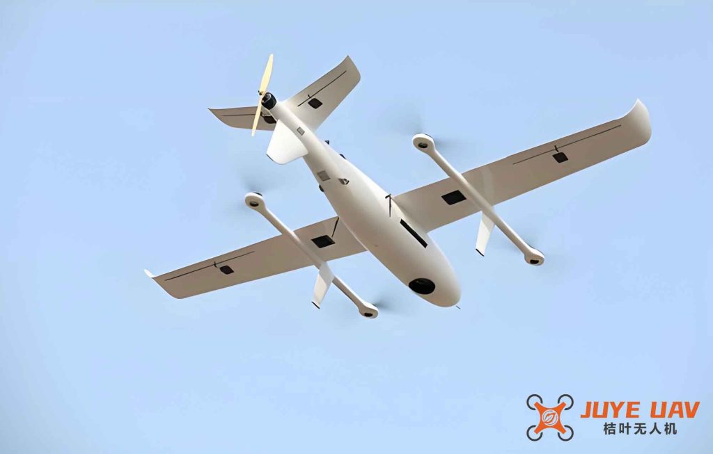
Figure 2 shows the time history of the tracking errors, confirming fixed-time convergence.
5. Conclusion
We have presented a distributed fixed-time formation tracking control algorithm for fixed-wing UAV swarms subject to actuator unmodeled dynamics and uncertainties. By leveraging a fixed-time terminal sliding mode, the controller guarantees that the swarm achieves the desired formation within a fixed time that is independent of initial conditions. The robust term compensates for external disturbances. Lyapunov analysis proves fixed-time stability, and numerical simulations with a three-UAV swarm confirm the effectiveness and robustness of the approach. Our method is particularly suitable for time-critical missions such as formation reconfiguration for obstacle avoidance. Future work will extend the results to directed communication topologies and time-varying formation requirements.
References (selected, formatted in IEEE style)
[1] S.-J. Chung, A. A. Paranjape, P. Dames, et al., “A survey on aerial swarm robotics,” IEEE Trans. Robot., vol. 34, no. 4, pp. 837–855, 2018.
[2] Z. Zuo, “Nonsingular fixed-time terminal sliding mode control of nonlinear systems,” IET Control Theory Appl., vol. 9, no. 4, pp. 545–552, 2015.
[3] B. Tian, Z. Zuo, and H. Wang, “Leader-follower fixed-time consensus of multi-agent systems with high-order integrator dynamics,” Int. J. Control, vol. 90, no. 7, pp. 1420–1427, 2017.
[4] W. Sui, “Distributed fixed-time coordinated control for spacecraft formation flying,” Ph.D. dissertation, Harbin Institute of Technology, 2020.
[5] Q. Dong, Y. Liang, and Y. Zhao, “UAV swarm formation control based on adaptive finite-time observer disturbance,” Sci. Sin. Technol., vol. 50, no. 4, pp. 423–438, 2020.