
In this paper, we investigate the guidance control problem of a small-to-medium-sized fixed-wing drone operating under wind disturbances. We propose an improved path following guidance algorithm that replaces the conventional PID-based lateral guidance law with a vector-field-based approach. By integrating this lateral algorithm with a PID longitudinal controller, we achieve significant enhancements in trajectory tracking accuracy and wind disturbance rejection. Through digital simulations and hardware-in-the-loop experiments, we demonstrate the effectiveness and superiority of the proposed method. The results show that the fixed-wing drone exhibits faster convergence, smaller cross-track errors, and smoother flight behavior, even in the presence of constant wind fields.
1. Introduction
Unmanned aerial vehicles (UAVs) are generally classified into consumer-grade and industrial-grade categories. While consumer drones are primarily used for entertainment and photography, industrial fixed-wing drones serve critical roles in terrain mapping, search and rescue, and military missions. One key capability enabling these applications is precise path following—the ability to autonomously track a predefined flight route. Before each mission, a ground station uploads a sequence of waypoints and path segments to the flight control system, and the fixed-wing drone must accurately follow these trajectories despite environmental perturbations such as wind.
Path following techniques can be broadly categorized into geometric methods and control-theoretic methods. Geometric approaches include pursuit guidance, line-of-sight (LOS) guidance, and vector field methods. Control-based methods range from classical PID to advanced nonlinear controllers such as LQR, sliding mode control, model predictive control, and adaptive control. Among these, the vector field method has gained attention due to its intuitive structure and robustness against wind. In particular, previous comparative studies have shown that vector field guidance outperforms other strategies under windy conditions.
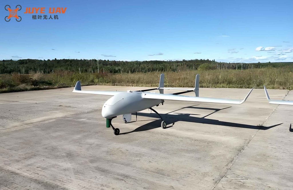
In this work, we focus on a specific small-to-medium-sized fixed-wing drone. We design a lateral guidance algorithm based on a vector field that uses only the cross-track error as the input to generate the desired course angle command. This algorithm replaces the original PID-based lateral guidance and is fused with a PID longitudinal altitude controller. We validate the algorithm through both numerical simulations and hardware-in-the-loop tests, confirming its superiority in wind-disturbed environments.
2. Problem Formulation
2.1 Fixed-Wing Drone Modeling
The fixed-wing drone considered in this study has a conventional autopilot architecture consisting of inner stability loops and outer guidance loops. The lateral and longitudinal dynamics are simplified as second-order systems. The simplified block diagrams are shown conceptually in the description, but here we present the mathematical model directly. The kinematics and dynamics for lateral motion are given by:
$$
\ddot{\chi} = \frac{g k_{P\chi}}{\| \mathbf{V}_g \|} (\dot{\chi}_c – \dot{\chi}) + \frac{g k_{I\chi}}{\| \mathbf{V}_g \|} (\chi_c – \chi) = a_{\dot{\chi}} (\dot{\chi}_c – \dot{\chi}) + a_{\chi} (\chi_c – \chi)
$$
where \(\chi\) is the course angle, \(\chi_c\) is the commanded course angle, \(\mathbf{V}_g\) is the ground velocity vector, \(g\) is the gravitational acceleration, and \(k_{P\chi}, k_{I\chi}\) are gains. The longitudinal dynamics for altitude hold are:
$$
\ddot{h} = \| \mathbf{V}_a \| k_{Ph} (\dot{h}_c – \dot{h}) + \| \mathbf{V}_a \| k_{Ih} (h_c – h) = a_{\dot{h}} (\dot{h}_c – \dot{h}) + a_h (h_c – h)
$$
where \(h\) is altitude, \(\mathbf{V}_a\) is the airspeed vector, and \(k_{Ph}, k_{Ih}\) are gains. The roll command \(\phi_c\) and pitch command \(\theta_c\) are generated as:
$$
\phi_c = k_{P\chi} (\chi_c – \chi) + \frac{k_{I\chi}}{s} (\chi_c – \chi)
$$
$$
\theta_c = k_{Ph} (h_c – h) + \frac{k_{Ih}}{s} (h_c – h)
$$
In this work, the altitude command \(h_c\) is typically a constant set by the mission plan, while the course command \(\chi_c\) is computed in real time by the lateral guidance algorithm. Therefore, the lateral path following problem is the main focus.
2.2 Path Following Geometry
The flight path consists of straight line segments and circular arcs. For a straight line segment, the cross-track error \(e_{Py}\) is the perpendicular distance from the fixed-wing drone to the desired path. As shown in the problem description, the position errors are transformed using the rotation matrix:
$$
\begin{bmatrix} \dot{e}_{Px} \\ \dot{e}_{Py} \end{bmatrix} = \begin{bmatrix} \cos\chi_q & \sin\chi_q \\ -\sin\chi_q & \cos\chi_q \end{bmatrix} \| \mathbf{V}_g \| \begin{bmatrix} \cos\chi \\ \sin\chi \end{bmatrix} = \| \mathbf{V}_g \| \begin{bmatrix} \cos(\chi – \chi_q) \\ \sin(\chi – \chi_q) \end{bmatrix}
$$
For a circular arc with radius \(\rho\), the radial distance \(d\) and its rate are:
$$
\dot{d} = \| \mathbf{V}_g \| \cos(\chi – \phi)
$$
$$
\dot{\phi} = \frac{\| \mathbf{V}_g \|}{d} \sin(\chi – \phi)
$$
where \(\phi\) is the phase angle relative to the circle center. The objective is to drive \(e_{Py} \to 0\) for straight lines and \(d \to \rho\) for arcs, with small steady-state errors and fast convergence.
3. Path Following Algorithm Design
3.1 PID-Based Guidance (Baseline)
For completeness, we first describe the original PID lateral guidance used in our fixed-wing drone. The roll command is computed as:
$$
\phi_c = k_{P\chi} \| \mathbf{V}_g \| \Delta\chi – k_{DP} D – k_{DI} \int D \, dt
$$
where \(\Delta\chi = \chi_q – \chi\) is the heading error for straight lines (or \(\chi_o – \chi\) for arcs), and \(D\) is the cross-track error (for straight lines \(D = e_{Py}\), for arcs \(D = d – \rho\)). Gains \(k_{P\chi}, k_{DP}, k_{DI}\) are tuned. The longitudinal PID altitude control is:
$$
\theta_c = k_{\theta P} (h_c – h) + k_{\theta I} \int (h_c – h) dt + k_{\theta D} \dot{h}
$$
3.2 Vector Field Lateral Guidance (Proposed)
The vector field method generates a desired course angle \(\chi_c\) based solely on the cross-track error, without needing the heading error explicitly. The key idea is to construct a vector field that points directly toward the path when the fixed-wing drone is far away, and aligns with the path direction when the drone is on the path.
3.2.1 Straight Line Path Following
Define the desired course angle as a function of the cross-track error \(e_{Py}\):
$$
\chi_c(e_{Py}) = -\arctan(k_m e_{Py}) + \chi_q
$$
where \(k_m\) is a positive constant that controls the transition rate from the approach angle to the path direction. When \(e_{Py}\) is large, \(\chi_c \approx \chi_q \pm \pi/2\) (depending on sign), directing the fixed-wing drone toward the path. When \(e_{Py} = 0\), \(\chi_c = \chi_q\). To avoid angle wrapping issues (when \(|\chi_c – \chi| > \pi\)), we apply a modulo operation:
$$
\chi_q = \arctan\left(\frac{q_e}{q_n}\right) + 2\pi n, \quad n \in \mathbb{N}, \text{ such that } |\chi_c – \chi| < \pi
$$
where \((q_n, q_e)\) is the unit direction vector of the path.
3.2.2 Circular Arc Path Following
For a circular arc of radius \(\rho\) and center \((c_n, c_e)\), the desired course angle is:
$$
\chi_c(d, \rho, \lambda) = \lambda \arctan\left( k_n \frac{d – \rho}{\rho} \right) + \chi_o
$$
where \(d\) is the distance from the fixed-wing drone to the circle center, \(\chi_o = \phi + \lambda \pi/2\) is the tangential course angle on the arc, \(\lambda = 1\) for clockwise and \(\lambda = -1\) for counterclockwise, and \(k_n\) is a gain. As before, a phase unwrapping procedure is applied when \(\phi\) jumps by \(2\pi\):
$$
\phi = \arctan(p_e – c_e, p_n – c_n) + 2\pi m, \quad m \in \mathbb{N}, \text{ such that } |\chi_c – \chi| < \pi
$$
The vector field method provides a smooth transition from a distant approach to path adherence. Table 1 summarizes the core equations for both algorithms.
| Algorithm | Command Generation | Input Variables |
|---|---|---|
| PID (Baseline) | \(\phi_c = k_{P\chi} \|V_g\| \Delta\chi – k_{DP} D – k_{DI} \int D dt\) | \(\Delta\chi, D\) |
| Vector Field (Proposed) | \(\chi_c = -\arctan(k_m e_{Py}) + \chi_q\) (straight) \(\chi_c = \lambda \arctan(k_n \frac{d-\rho}{\rho}) + \chi_o\) (arc) |
\(e_{Py}\) (straight), \(d\) (arc) |
4. Simulation and Experimental Results
4.1 Digital Simulation Setup
We conducted digital simulations in MATLAB/Simulink with a step size of 0.01 s. The fixed-wing drone model parameters are: \(a_{\chi} = 0.732\), \(a_{\dot{\chi}} = 5.968\). The PID gains are: \(k_{P\chi} = 0.105\), \(k_{DP} = 1.815\), \(k_{DI} = 0.006\). For the vector field method, we set \(k_m = 0.05\), \(k_n = 8\). The roll command is saturated at \(\pm 35^\circ\) with a rate limit of \(\pm 35^\circ/\text{s}\). A constant wind of 6 m/s from 315° is applied. The airspeed is 20 m/s.
4.2 Straight Line Path Following – Short Initial Offset
The target line is \(y = 0\) (north direction). The fixed-wing drone starts at \((0, 100)\) m with initial heading 90°. Figure 1 in the original paper is replaced here by simulation data tables. Table 2 presents the key performance metrics.
| Metric | PID | Vector Field |
|---|---|---|
| Settling time to 2.1 m error (s) | 54 | 30 |
| Steady-state cross-track error (m) | 2.1 | 2.1 |
| Overshoot in cross-track | Moderate | Minimal |
| Course angle stability | Oscillatory | Smooth |
4.3 Straight Line Path Following – Long Initial Offset
Starting at \((0, 400)\) m, the fixed-wing drone must converge to the same line. The vector field method shows a clear advantage in convergence distance and time, as shown in Table 3.
| Metric | PID | Vector Field |
|---|---|---|
| Settling time to stable heading (s) | 77 | 46 |
| Steady-state cross-track error (m) | 5.5 | 3.5 |
| Roll angle oscillations | Significant | Negligible |
4.4 Circular Arc Path Following
The path consists of two semicircles of radius 200 m. The fixed-wing drone starts at \((0, 200)\) m. The vector field approach reduces total mission time and tracking error. Table 4 summarizes the results.
| Metric | PID | Vector Field |
|---|---|---|
| Total flight time for arc segment (s) | 81 | 74 |
| Maximum radial error in second half (m) | >10 (oscillatory) | <3 |
| Course angle smoothness | Oscillations at transition | Very smooth |
4.5 Hardware-in-the-Loop Simulation
We performed a hardware-in-the-loop (HIL) simulation using the actual flight controller of our fixed-wing drone. The simulation environment included a six-degree-of-freedom model, engine model, and constant wind of 6 m/s from 45°. The drone was launched via catapult and flew a predefined route consisting of straight legs and turns. The vector field lateral guidance was active throughout.
The HIL results confirmed stable path following with smooth transitions. The altitude hold using PID also performed well. The cross-track error remained below 5 m for straight segments and below 8 m for turns. No oscillations or divergence were observed. The algorithm was validated for several runs with different wind conditions. Table 5 provides key data from one representative HIL test.
| Parameter | Value |
|---|---|
| Straight segment max cross-track error (m) | 4.2 |
| Turn segment max cross-track error (m) | 7.8 |
| Altitude error (m) (RMS) | 1.5 |
| Roll angle oscillations | None |
| Course angle tracking | Accurate |
The fixed-wing drone’s path overlapped closely with the planned trajectory, demonstrating the practical applicability of the vector field method.
5. Conclusion
We have designed and implemented a vector field-based lateral guidance algorithm for a small-to-medium-sized fixed-wing drone operating in windy environments. By generating the desired course angle directly from the cross-track error, the algorithm eliminates the need for explicit heading error feedback and provides smoother convergence. Digital simulations show that the proposed method reduces settling time by up to 40% and steady-state error by up to 36% compared to the traditional PID lateral guidance. The fixed-wing drone exhibits less roll oscillation and more stable course tracking under constant wind disturbances. Hardware-in-the-loop experiments confirm that the vector field algorithm integrates seamlessly with the existing PID longitudinal controller, resulting in reliable autonomous path following. This work provides a practical and effective solution for enhancing the wind rejection capability of fixed-wing drones in real-world missions.