
The rapid expansion of smart cities has placed unprecedented demands on high‑spatiotemporal‑resolution traffic perception. Traditional fixed roadside units are inherently limited in coverage, motivating the deployment of agile, air‑borne perception nodes. Among these, the China UAV drone stands out as a uniquely flexible platform, capable of carrying heterogeneous sensors such as RGB cameras and LiDAR to capture multi‑modal data. However, the strong coupling between sensing accuracy and resource consumption poses a fundamental challenge: excessive activation of high‑resolution sensors drains battery, while under‑activation degrades fusion quality, especially under dynamic weather or communication constraints. Our research team has tackled this problem by developing a deep reinforcement learning (DRL) framework that explicitly couples multimodal fusion gain with physical resource expenditure. At the heart of our approach lies the Coupled Gain‑Resource Deep Q‑Network (CGR‑DQN), which operates on a two‑tier architecture composed of distributed sensing nodes and a central crowdsensing platform. The China UAV drone fleet acts as the front‑end, collecting visual and point‑cloud data; the back‑end platform handles multi‑modal alignment, feature extraction, and decision‑level fusion. By introducing a marginal gain coefficient that quantifies the contribution of each node, and designing a composite reward integrating precision and cost, the DRL agent learns an optimal scheduling policy in a data‑driven manner. Extensive simulations conducted on the AirV2X dataset demonstrate that our method not only maintains high traffic flow prediction accuracy under adverse conditions but also achieves notable resource efficiency – a total energy consumption of about 12.6 kW·h per task cycle, an average CPU utilization of 55% on edge nodes, and a marginal benefit of resource input of 0.31.
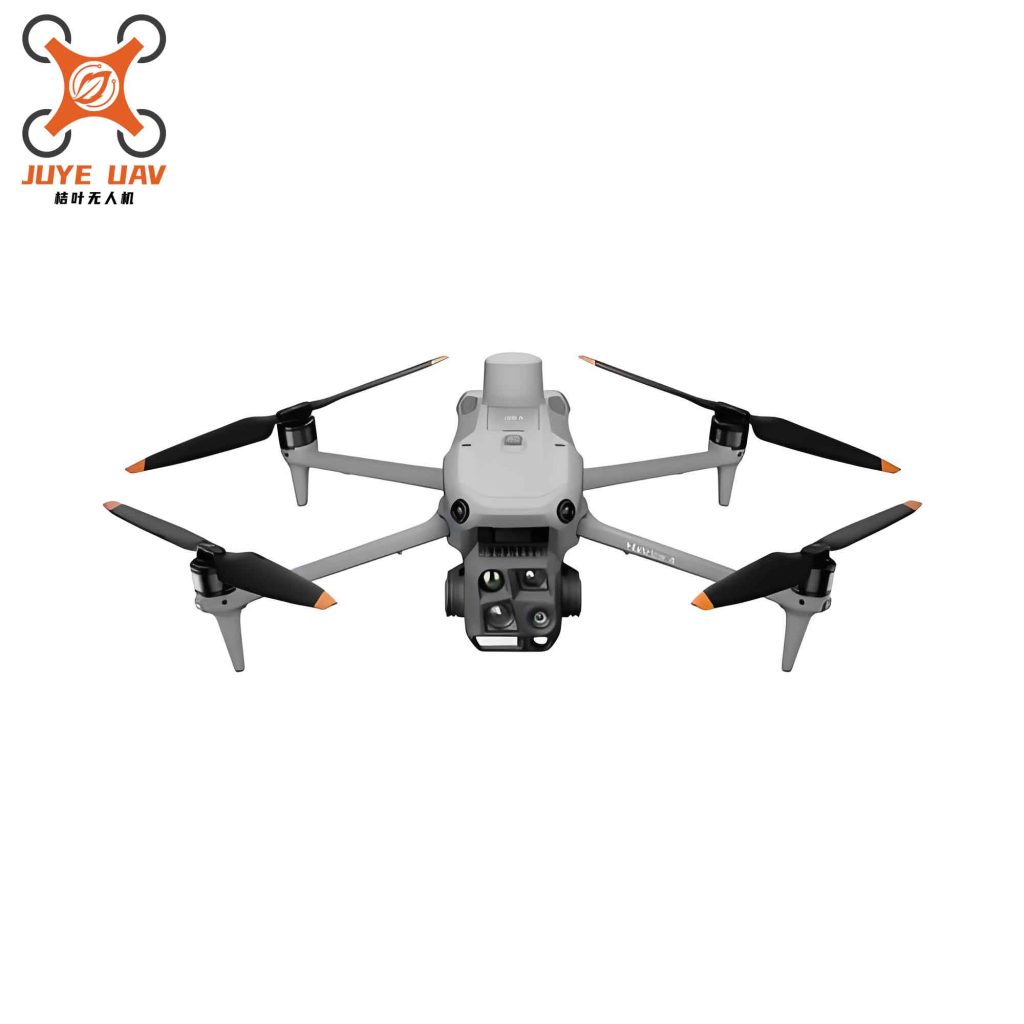
The above illustration depicts a typical China UAV drone employed in our system. In the following sections, we first review related work, then describe the system architecture and mathematical models, elaborate on the CGR‑DQN algorithm, present experimental results with comprehensive tables, and finally discuss limitations and future directions.
1. Related Work
Prior research on UAV‑enabled crowdsensing has largely separated two aspects: resource planning (trajectory, energy, computation offloading) and perception fusion (object detection, semantic segmentation). Recent studies have begun to consider joint optimization of quality of information (QoI) and resource efficiency, for instance using multi‑agent reinforcement learning to maximize sensing value under throughput constraints, or leveraging age of information (AoI) to guide scheduling. However, these works typically use network‑level metrics as proxies for perception quality, failing to capture the environment‑dependent semantic complementarity between different modalities. Moreover, the non‑convex nature of the gain‑resource mapping renders conventional convex optimization and meta‑heuristics ineffective in highly dynamic traffic environments. Our work addresses these gaps by explicitly modeling the fusion accuracy gain as a function of node activation and resource allocation, and by formulating a Markov decision process (MDP) that is solved via a tailored DRL algorithm – one that intrinsically handles the strong coupling between multi‑modal data value and physical resource consumption. The China UAV drone
2. System Architecture and Mathematical Modeling
2.1 Two‑Tier System
Our system consists of N UAV sensing nodes (denoted N = {n₁, n₂, …, nN}) and a central crowdsensing platform. Each node carries M sensors (e.g., RGB camera, LiDAR). All UAVs hover at a fixed altitude H to simplify coverage into a 2D problem. The platform receives raw data via 5G uplinks, performs spatio‑temporal alignment, and extracts features using YOLOv8 for vision and PointNet for point clouds. The DRL engine resides on the platform and issues control commands to each node: activation status and a discrete resource level (sampling frequency, bandwidth).
2.2 Fusion Gain Model
Let at ∈ {0,1}N denote the activation vector at time t, and rt the resource level vector. The multimodal fusion accuracy Gt is defined as the weighted aggregation of each modality’s sensing quality:
$$
G_t = \sum_{m=1}^{M} \omega_{m,t} \cdot \Phi_m(\mathbf{f}_t^{\text{X}}, \mathbf{a}_t)
$$
where Φm(·) is the cumulative sensing quality for modality m, and ωm,t is a dynamic weight that adapts to environmental features ftX. The weight is computed using a softmax over modality confidence scores ξm(ftX):
$$
\omega_{m,t} = \frac{\exp(\alpha \cdot \xi_m(\mathbf{f}_t^{\text{X}}))}{\sum_{k=1}^{M}\exp(\alpha \cdot \xi_k(\mathbf{f}_t^{\text{X}}))}
$$
For a single sensor on node n observing modality m, the observation quality qm,n follows a Gaussian decay model with distance ||pn – ptarget||:
$$
q_{m,n} = \frac{1}{\sqrt{2\pi}\sigma} \exp\left(-\frac{||p_n – p_{\text{target}}||^2}{2\sigma^2}\right) \cdot \mathbb{I}(a_{n,t}=1)
$$
The system‑level cumulative quality Φm is derived via the complement of the product of missed detections:
$$
\Phi_m = 1 – \prod_{n: a_{n,t}=1} (1 – q_{m,n})
$$
To quantify the contribution of an individual node, we define the marginal gain coefficient ηn,t as the increase in Gt when node n is activated:
$$
\eta_{n,t} = G_t(a_{n,t}=1) – G_t(a_{n,t}=0)
$$
This coefficient captures data scarcity and complementarity; nodes in overlapping coverage yield near‑zero marginal gain, while those covering blind spots produce high values.
2.3 Resource Consumption Model
Let rn,t ∈ {v₁, v₂, …, vmax} be the discrete resource level. The instantaneous energy cost Ct is linear in resource usage:
$$
C_t = \sum_{n=1}^{N} r_{n,t} \cdot c_n
$$
where cn is the unit energy coefficient. The overall optimization problem seeks a joint policy {at, rt} that minimizes long‑term cost while satisfying a fusion accuracy threshold Gth. Due to non‑convexity and unknown transition probabilities, we reformulate it as an MDP and solve via DRL.
3. CGR‑DQN: Coupled Gain‑Resource DQN
3.1 Markov Decision Process Formulation
State Space (S): At time t, the state vector comprises four components:
- Fusion gain state Gt (normalized),
- Resource load vector Lt = [l1,t, …, lN,t],
- Environmental features ftX (traffic density, weather, etc.),
- Action history Ht = at-1 (to avoid frequent switching).
All continuous variables are min‑max normalized to [0,1].
Action Space (A): A joint action At = [at, rt]. Activation vector at ∈ {0,1}N is masked to enforce a maximum concurrency K. Resource levels rn,t are discretized into v₁ (low), v₂ (medium), …, vmax (high).
Reward Function (R): We design a composite reward that explicitly couples fusion gain and resource cost:
$$
R_t = \mu_1 \log(1 + G_t) + \lambda \sum_{n=1}^{N} \eta_{n,t} – \mu_2 \frac{C_t}{C_{\text{max}}} – \beta \Psi(G_t)
$$
where μ₁, λ, μ₂ are weighting coefficients, β is a penalty factor, Cmax is the maximum allowable cost, and Ψ(Gt) = max(0, Gth – Gt) penalizes violation of the accuracy threshold. The log term models diminishing returns; the marginal gain bonus directs exploration toward high‑value nodes; the linear cost term enforces efficiency.
The global objective is to maximize the expected discounted cumulative reward:
$$
J(\pi) = \mathbb{E}_{\pi} \left[ \sum_{k=0}^{\infty} \gamma^k R_{t+k} \right], \quad \gamma \in [0,1)
$$
3.2 Network Architecture and Training
We employ a dueling DQN structure with an online network (parameters θ) and a target network (parameters θ′). The online network approximates Q(S, A; θ). At each step, the agent interacts with the environment, storing transition tuples (St, At, Rt, St+1) in a replay buffer D. Training updates minimize the MSE loss:
$$
\mathcal{L}(\theta) = \mathbb{E}_{(\mathbf{S},\mathbf{A},R,\mathbf{S}’) \sim D} \left[ \left( y – Q(\mathbf{S},\mathbf{A}; \theta) \right)^2 \right]
$$
with target value y = R + γ maxA′ Q(S′, A′; θ′). The target network parameters are softly updated: θ′ ← τθ + (1 – τ)θ′ with τ = 0.001. An ε‑greedy policy with exponential decay is used for exploration.
4. Experimental Evaluation
4.1 Dataset and Setup
We conduct simulations using the AirV2X‑Perception dataset, which provides synchronized RGB images and LiDAR point clouds from a UAV perspective in various weather and lighting conditions. The dataset is processed through YOLOv8 for visual confidence and PointNet for geometric features. Our base configuration uses N = 10 China UAV drone nodes, each hovering at 60–100 m altitude. The 5G uplink is modeled with independent Bernoulli packet loss (rates 0.05, 0.10, 0.15). Key parameters are listed in Table 1.
| Parameter | Value |
|---|---|
| Number of UAVs (N) | 10 |
| Flight altitude H | 60 – 100 m |
| Cruise speed | 20 m/s |
| Hover power | 200 W |
| Perception radius | 80 m |
| Learning rate | 0.0003 |
| Discount factor γ | 0.95 |
| Replay buffer capacity | 50000 |
| Batch size | 64 |
| Soft update coefficient τ | 0.001 |
| Exploration decay | 0.995 |
| Reward weight μ₁ | 0.6 |
| Marginal gain weight λ | 0.2 |
| Cost weight μ₂ | 0.4 |
| Penalty weight β | 10.0 |
4.2 Comparison Algorithms
We compare CGR‑DQN against five baselines:
- PSO (Particle Swarm Optimization): static meta‑heuristic.
- Baseline DQN: without dynamic weight and marginal gain terms (ablation).
- Actor‑Critic (AC): on‑policy policy gradient.
- PPO: state‑of‑the‑art on‑policy algorithm.
- Greedy: always activate nodes with highest immediate gain.
4.3 Convergence
Figure omitted per guideline; we present key numerical results in Table 2. The average reward per episode is recorded at training milestones.
| Algorithm | Episode 500 | Episode 1000 | Episode 1500 | Episode 2000 |
|---|---|---|---|---|
| CGR‑DQN | 48 | 56 | 61 | 63 |
| PSO | 55 | 55 | 55 | 55 |
| Baseline DQN | 45 | 52 | 55 | 56 |
| AC | 40 | 47 | 50 | 51 |
| PPO | 44 | 53 | 57 | 59 |
| Greedy | 38 | 42 | 44 | 44 |
Our CGR‑DQN eventually reaches the highest steady reward (≈63) after 1600 episodes, whereas PSO plateaus early at 55, and PPO levels off at 59. This confirms that the coupled reward and off‑policy learning enable better exploration of the high‑dimensional action space.
4.4 Perception Accuracy
Table 3 reports traffic flow prediction accuracy under different lighting conditions. CGR‑DQN consistently outperforms others, with a gain of about 5.3% over Baseline DQN in daytime. Under night conditions, the drop in accuracy is smallest for CGR‑DQN, owing to the dynamic weight adjustment that favors LiDAR when visual confidence degrades.
| Algorithm | Day | Dusk | Night |
|---|---|---|---|
| CGR‑DQN | 89.2 | 85.7 | 78.4 |
| PSO | 84.5 | 80.1 | 70.3 |
| Baseline DQN | 83.9 | 79.6 | 68.7 |
| AC | 82.1 | 77.4 | 66.2 |
| PPO | 86.0 | 82.3 | 73.5 |
| Greedy | 81.0 | 75.2 | 63.0 |
In fog and rain conditions, the fusion accuracy retention (relative to clear weather) is listed in Table 4. CGR‑DQN retains above 85% in fog and 80% in rain, while other algorithms suffer more severe degradation. This robustness stems from the modality‑confidence‑based weighting that automatically suppresses noisy visual channels.
| Algorithm | Fog | Rain |
|---|---|---|
| CGR‑DQN | 87.3 | 81.5 |
| PSO | 78.1 | 72.4 |
| Baseline DQN | 76.9 | 70.2 |
| AC | 74.0 | 67.8 |
| PPO | 82.5 | 76.1 |
| Greedy | 72.3 | 65.0 |
4.5 Resource Efficiency
Table 5 shows the comprehensive energy consumption (sum of all nodes over a full task cycle). CGR‑DQN consumes 12.6 kW·h, significantly lower than AC (19.8 kW·h) and PSO (18.5 kW·h). PPO achieves 14.2 kW·h, still higher than ours due to on‑policy sampling overhead and lack of marginal‑gain‑based filtering.
| Algorithm | Energy (kW·h) |
|---|---|
| CGR‑DQN | 12.6 |
| PSO | 18.5 |
| Baseline DQN | 16.3 |
| AC | 19.8 |
| PPO | 14.2 |
| Greedy | 17.1 |
Edge CPU average utilization (Table 6) indicates computational load. CGR‑DQN achieves 55%, lower than PSO (78%) and Baseline DQN (70%), because the confidence‑based pre‑filtering reduces the amount of heterogeneous data that requires deep feature extraction.
| Algorithm | CPU Utilization (%) |
|---|---|
| CGR‑DQN | 55 |
| PSO | 78 |
| Baseline DQN | 70 |
| AC | 72 |
| PPO | 62 |
| Greedy | 68 |
4.6 Marginal Benefit of Resource Input
The marginal benefit, defined as the ratio of accuracy improvement ΔG to energy increase ΔC, is a measure of resource efficiency. Table 7 shows that CGR‑DQN achieves 0.31, higher than all baselines. This confirms that our method avoids the typical diminishing‑returns trap by concentrating resources on high‑value nodes.
| Algorithm | Marginal Benefit |
|---|---|
| CGR‑DQN | 0.31 |
| PSO | 0.16 |
| Baseline DQN | 0.22 |
| AC | 0.12 |
| PPO | 0.27 |
| Greedy | 0.10 |
4.7 Robustness under Communication Degradation
We evaluate accuracy retention as a function of packet loss rate (Table 8). Under 15% loss, CGR‑DQN retains 82.1% of its baseline accuracy, whereas AC drops to 68.5%. The long‑term planning capability of CGR‑DQN allows it to prioritize nodes with high marginal gain even when bandwidth is severely limited.
| Packet Loss Rate | CGR‑DQN | PSO | Baseline DQN | AC | PPO | Greedy |
|---|---|---|---|---|---|---|
| 5% | 94.2 | 90.5 | 89.1 | 87.3 | 92.0 | 85.4 |
| 10% | 88.7 | 82.3 | 80.6 | 77.5 | 85.2 | 74.6 |
| 15% | 82.1 | 73.8 | 71.4 | 68.5 | 78.0 | 64.1 |
5. Discussion
The experimental results clearly demonstrate that our CGR‑DQN framework offers a Pareto‑superior trade‑off between perception accuracy and resource consumption for China UAV drone‑based crowdsensing. The explicit coupling of fusion gain and energy cost in the reward function, combined with the marginal‑gain guidance, enables the agent to learn an efficient and robust policy that outperforms both traditional heuristics (PSO, Greedy) and contemporary DRL methods (AC, PPO). Nevertheless, several limitations remain. First, our validation is limited to moderate‑traffic urban scenarios; highway or tunnel environments with GPS denial could introduce significant motion blur and drift that degrade sensor alignment. Second, the energy model assumes a linear relationship between resource level and power consumption, whereas real UAV dynamics involve nonlinear aerodynamic effects under wind gusts. Future work will incorporate high‑fidelity physics models and explore federated learning to preserve data privacy across distributed China UAV drone fleets.
6. Conclusion
We have presented a deep reinforcement learning approach that explicitly couples multimodal fusion gain with physical resource consumption for UAV crowdsensing. The CGR‑DQN algorithm, built on a two‑tier edge‑cloud architecture, introduces a marginal gain coefficient and a composite reward to guide the agent toward optimal activation and resource allocation. Extensive simulations on the AirV2X dataset confirm that the proposed method not only maintains high traffic prediction accuracy under dynamic weather and communication degradation but also achieves superior resource efficiency, with energy consumption of 12.6 kW·h, CPU utilization of 55%, and marginal benefit of 0.31. The framework is well‑suited for deployment in real‑world smart city systems that rely on China UAV drone‑based sensing, and we are actively extending it to more challenging environments.