
In the rapidly evolving field of unmanned aerial systems, the development of a reliable and autonomous quadrotor drone presents a fascinating and complex engineering challenge. My journey into designing a simulation control system for such a platform begins with acknowledging the core difficulties: establishing an accurate dynamic model amidst real-world disturbances, designing a controller for an inherently unstable, underactuated, and strongly coupled system, and effectively utilizing sensor feedback for stable autonomy. This document details my first-person approach to tackling these problems, focusing on dynamics modeling, linearization, and PID controller design within a simulation environment, laying a robust foundation for physical implementation. The term quadrotor drone will be central to our discussion, representing the specific type of UAV under investigation.
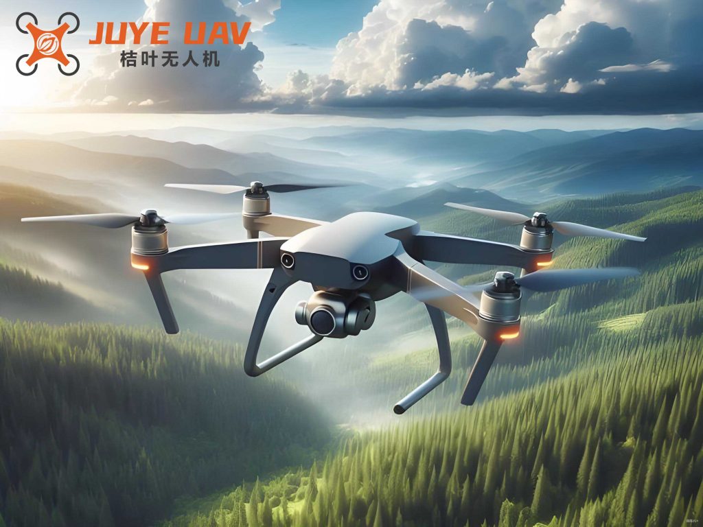
The fundamental flight principle of a quadrotor drone is based on varying the rotational speeds of four independent rotors to generate lift and control moments. By manipulating these speeds in a coordinated manner, the drone can achieve lift, roll, pitch, and yaw motions. This simple mechanical structure belies a complex nonlinear dynamic behavior. To systematically design a controller, the first and most critical step is to derive a mathematical model that captures the essential physics of the quadrotor drone’s motion.
1. Kinematic and Dynamic Modeling of the Quadrotor Drone
To mathematically describe the motion of the quadrotor drone, I define two primary coordinate frames, as illustrated in the figure above. The Earth-Fixed Inertial Frame (E-frame), denoted by axes \(O_X Y Z\), is considered stationary. The Body-Fixed Frame (B-frame), denoted by axes \(O_{x_b y_b z_b}\), is attached to the center of mass of the drone. The orientation of the body frame relative to the inertial frame is described by three Euler angles: roll (\(\phi\)), pitch (\(\theta\)), and yaw (\(\psi\)). The rotation sequence is typically Z-Y-X (yaw, then pitch, then roll).
The transformation from the body frame to the inertial frame is accomplished by the rotation matrix \(^E\mathbf{R}_B\), which is a function of the Euler angles:
$$
^E\mathbf{R}_B = \begin{bmatrix}
c_\psi c_\theta & c_\psi s_\theta s_\phi – s_\psi c_\phi & c_\psi s_\theta c_\phi + s_\psi s_\phi \\
s_\psi c_\theta & s_\psi s_\theta s_\phi + c_\psi c_\phi & s_\psi s_\theta c_\phi – c_\psi s_\phi \\
-s_\theta & c_\theta s_\phi & c_\theta c_\phi
\end{bmatrix}
$$
where \(s_\cdot\) and \(c_\cdot\) denote \(\sin(\cdot)\) and \(\cos(\cdot)\), respectively.
For a standard quadrotor drone configuration, I assume the four rotors are aligned with the body \(z_b\)-axis. The thrust \(F_i\) generated by each rotor \(i\) is assumed to be proportional to the square of its rotational speed, \(F_i = k_F \omega_i^2\). The total thrust \(T\) is the sum of the individual thrusts. The reactive torque \(M_i\) generated by each rotor is also proportional to the square of its speed, \(M_i = k_M \omega_i^2\), and opposes the motor’s rotation. By strategically varying the speeds of diagonally opposite pairs of rotors, control moments are generated.
Applying Newton-Euler formalism, the translational and rotational dynamics of the quadrotor drone in the inertial frame can be derived. The translational dynamics are governed by:
$$
\begin{align*}
m \ddot{x} &= T(\cos\psi \sin\theta \cos\phi + \sin\psi \sin\phi) – K_{d,x} \dot{x} \\
m \ddot{y} &= T(\sin\psi \sin\theta \cos\phi – \cos\psi \sin\phi) – K_{d,y} \dot{y} \\
m \ddot{z} &= T\cos\theta \cos\phi – mg – K_{d,z} \dot{z}
\end{align*}
$$
The rotational dynamics are governed by:
$$
\begin{align*}
I_{xx}\ddot{\phi} &= \dot{\theta}\dot{\psi}(I_{yy} – I_{zz}) + l(F_4 – F_2) – K_{d,\phi} \dot{\phi} \\
I_{yy}\ddot{\theta} &= \dot{\phi}\dot{\psi}(I_{zz} – I_{xx}) + l(F_3 – F_1) – K_{d,\theta} \dot{\theta} \\
I_{zz}\ddot{\psi} &= \dot{\phi}\dot{\theta}(I_{xx} – I_{yy}) + (M_1 – M_2 + M_3 – M_4) – K_{d,\psi} \dot{\psi}
\end{align*}
$$
Where:
- \(m\) is the total mass of the quadrotor drone.
- \(g\) is the acceleration due to gravity.
- \(l\) is the distance from the center of mass to the axis of a rotor.
- \(I_{xx}, I_{yy}, I_{zz}\) are the moments of inertia.
- \(K_{d,*}\) are aerodynamic damping coefficients (often neglected for initial controller design near hover).
- \(T = F_1+F_2+F_3+F_4\) is the total thrust.
This model is highly nonlinear and coupled. The control inputs are the four rotor forces \(F_1, F_2, F_3, F_4\), but we have six degrees of freedom (position \(x,y,z\) and orientation \(\phi,\theta,\psi\)), making it an underactuated system. A common and effective simplification for control design is to consider the system’s behavior around a hover condition, where angles \(\phi\) and \(\theta\) are small (i.e., \(\sin(\alpha) \approx \alpha\), \(\cos(\alpha) \approx 1\)). Under this assumption, and neglecting damping and Coriolis terms for initial design, the dynamics simplify significantly and can be partially decoupled. It is convenient to define a virtual control input vector \(\mathbf{u}\):
$$
\begin{align*}
u_1 &= F_1 + F_2 + F_3 + F_4 \quad &\text{(Total Thrust)} \\
u_2 &= F_4 – F_2 \quad &\text{(Roll Moment Input)} \\
u_3 &= F_3 – F_1 \quad &\text{(Pitch Moment Input)} \\
u_4 &= F_1 – F_2 + F_3 – F_4 \quad &\text{(Yaw Moment Input)}
\end{align*}
$$
The simplified, linearized dynamics near hover become:
$$
\begin{align*}
\ddot{x} &= -g \theta \\
\ddot{y} &= g \phi \\
\ddot{z} &= \frac{u_1}{m} – g \\
\ddot{\phi} &= \frac{l}{I_{xx}} u_2 \\
\ddot{\theta} &= \frac{l}{I_{yy}} u_3 \\
\ddot{\psi} &= \frac{1}{I_{zz}} u_4
\end{align*}
$$
This decoupled representation is crucial for controller design, as it allows me to treat the altitude (\(z\)), roll (\(\phi\)), pitch (\(\theta\)), and yaw (\(\psi\)) channels independently. The translational motions (\(x, y\)) are directly coupled to the pitch and roll angles, respectively.
2. System Linearization and State-Space Representation
To apply linear control theory, I express the simplified dynamics in state-space form. For the attitude channels (roll, pitch, yaw), I define the state vector for each as its angle and angular rate. Taking the roll channel as an example, with state vector \(\mathbf{x}_\phi = [\phi, \dot{\phi}]^T\), the state-space equations are:
$$
\dot{\mathbf{x}}_\phi = \begin{bmatrix} 0 & 1 \\ 0 & 0 \end{bmatrix} \mathbf{x}_\phi + \begin{bmatrix} 0 \\ \frac{l}{I_{xx}} \end{bmatrix} u_2, \quad y_\phi = \begin{bmatrix} 1 & 0 \end{bmatrix} \mathbf{x}_\phi
$$
This is a double integrator system. A similar form holds for pitch (\(\theta\)) and yaw (\(\psi\)). For the altitude channel, with state \(\mathbf{x}_z = [z, \dot{z}]^T\), the equations are:
$$
\dot{\mathbf{x}}_z = \begin{bmatrix} 0 & 1 \\ 0 & 0 \end{bmatrix} \mathbf{x}_z + \begin{bmatrix} 0 \\ \frac{1}{m} \end{bmatrix} u_1 – \begin{bmatrix} 0 \\ g \end{bmatrix}, \quad y_z = \begin{bmatrix} 1 & 0 \end{bmatrix} \mathbf{x}_z
$$
To complete the plant model for simulation, I must include the actuator dynamics. Each brushless DC motor and propeller combination can be approximated as a first-order system relating the commanded input signal (e.g., PWM or voltage) to the generated thrust. Based on empirical data from a typical small quadrotor drone, this relationship can be modeled as:
$$
G_m(s) = \frac{K_m}{\tau s + 1}
$$
where \(K_m\) is the motor gain and \(\tau\) is the motor time constant. Therefore, the complete linear plant model \(G(s)\) for the decoupled altitude and attitude channels is a series connection of the motor dynamics and the double-integrator rigid-body dynamics. For a specific small quadrotor drone with parameters listed in the table below, the transfer functions are calculated.
| Parameter | Symbol | Value | Unit |
|---|---|---|---|
| Mass | \(m\) | 1.176 | kg |
| Gravity | \(g\) | 9.81 | m/s² |
| Arm Length | \(l\) | 0.26 | m |
| Roll Inertia | \(I_{xx}\) | 0.008 | kg·m² |
| Pitch Inertia | \(I_{yy}\) | 0.008 | kg·m² |
| Yaw Inertia | \(I_{zz}\) | 0.016 | kg·m² |
| Motor Gain | \(K_m\) | 0.78 | N/input |
| Motor Time Constant | \(\tau\) | 0.1 | s |
Using these parameters, the individual channel transfer functions become:
$$
\begin{align*}
G_z(s) &= \frac{\dot{Z}(s)}{U_1(s)} = \frac{K_m/m}{s(\tau s + 1)} = \frac{0.663}{s(0.1s + 1)} \\
G_\phi(s) &= \frac{\dot{\Phi}(s)}{U_2(s)} = \frac{l K_m / I_{xx}}{s(\tau s + 1)} = \frac{25.35}{s(0.1s + 1)} \\
G_\theta(s) &= \frac{\dot{\Theta}(s)}{U_3(s)} = \frac{l K_m / I_{yy}}{s(\tau s + 1)} = \frac{25.35}{s(0.1s + 1)} \\
G_\psi(s) &= \frac{\dot{\Psi}(s)}{U_4(s)} = \frac{K_m / I_{zz}}{s(\tau s + 1)} = \frac{48.75}{s(0.1s + 1)}
\end{align*}
$$
Where \(\dot{Z}, \dot{\Phi}, \dot{\Theta}, \dot{\Psi}\) are the Laplace transforms of the vertical velocity, roll rate, pitch rate, and yaw rate, respectively. The complete, decoupled MIMO plant model is:
$$
\mathbf{G}(s) = \begin{bmatrix}
G_z(s) & 0 & 0 & 0 \\
0 & G_\phi(s) & 0 & 0 \\
0 & 0 & G_\theta(s) & 0 \\
0 & 0 & 0 & G_\psi(s)
\end{bmatrix}
$$
3. PID Controller Design and Tuning
With a linearized and decoupled plant model for the quadrotor drone, I proceed to design Proportional-Integral-Derivative (PID) controllers for each channel. The PID controller is a robust and widely understood algorithm, making it an excellent starting point for stabilizing a quadrotor drone. The continuous-time transfer function of a PID controller is:
$$
C(s) = K_p + \frac{K_i}{s} + K_d s = K_p \left(1 + \frac{1}{T_i s} + T_d s\right)
$$
where \(K_p\) is the proportional gain, \(K_i\) is the integral gain, \(K_d\) is the derivative gain, \(T_i = K_p/K_i\) is the integral time, and \(T_d = K_d/K_p\) is the derivative time.
The control objective for each attitude channel is to make the angle (\(\phi, \theta, \psi\)) track a desired reference (often zero for hover) quickly and with minimal overshoot, rejecting disturbances like wind gusts. The altitude controller aims to maintain or track a desired height. The control structure for one channel in Simulink is straightforward: the error between the desired state and the measured state is fed into the PID controller, whose output drives the plant.
I employ a systematic tuning approach, starting with the Ziegler-Nichols frequency response method as a guideline to find initial gain values. The process involves:
- Setting \(K_i = 0\) and \(K_d = 0\).
- Increasing \(K_p\) until the system output exhibits sustained oscillations (the ultimate gain \(K_u\)). The period of these oscillations is the ultimate period \(P_u\).
- Using Ziegler-Nichols formulas to compute initial PID parameters: \(K_p = 0.6K_u\), \(T_i = 0.5P_u\), \(T_d = 0.125P_u\).
However, for a quadrotor drone simulation, I often need to adjust these values heuristically within the simulation environment to meet specific performance criteria such as rise time, settling time, overshoot, and disturbance rejection. The derivative term is particularly sensitive and must be chosen carefully to avoid amplifying high-frequency noise. A practical step is to filter the derivative action, implementing a “real” derivative term: \(K_d s / (1 + T_f s)\), where \(T_f\) is a small filter time constant.
After iterative simulation and tuning, I arrived at a set of PID parameters that provide stable and responsive control for the simulated quadrotor drone. The performance of each controller was evaluated against step inputs and impulse disturbances.
| Control Channel | Proportional Gain \(K_p\) | Integral Gain \(K_i\) | Derivative Gain \(K_d\) | Derivative Filter \(T_f\) (s) |
|---|---|---|---|---|
| Altitude (Z) | 3.2 | 0.8 | 1.5 | 0.01 |
| Roll (\(\phi\)) | 2.5 | 0.02 | 0.75 | 0.01 |
| Pitch (\(\theta\)) | 2.5 | 0.02 | 0.75 | 0.01 |
| Yaw (\(\psi\)) | 4.8 | 0.04 | 1.40 | 0.01 |
4. Simulation Framework and Performance Analysis
I constructed a comprehensive nonlinear simulation model in MATLAB/Simulink to validate the controller design. The model integrates several key components:
- Nonlinear Plant Model: This block implements the full 6-DOF nonlinear equations of motion derived in Section 1, including the gravitational force and the mapping from rotor forces to moments.
- Actuator Model: A first-order lag for each motor, converting the controller’s force command into a simulated rotor thrust.
- PID Controller Bank: Four independent PID controllers (one for each channel: Z, \(\phi\), \(\theta\), \(\psi\)) with the parameters from Table 2.
- Command Generator: Provides reference signals for hover (zero roll, pitch, yaw, constant altitude) or maneuver sequences.
- Disturbance Injection: Allows the application of step or gust disturbances to the attitude angles or forces, simulating wind or weight imbalance.
The primary test scenario is hover stabilization. The simulation initializes the quadrotor drone at a non-zero attitude (e.g., 0.2 rad roll) and/or with an altitude error. The controllers must drive all states to zero. A more rigorous test involves applying an external step disturbance (e.g., a momentary torque simulating a wind gust) after the drone has stabilized and observing the recovery.
The simulation results demonstrated the effectiveness of the designed PID controllers. For a step disturbance in roll angle, the controller successfully returned the quadrotor drone to a level attitude. Key performance metrics extracted from the simulations are summarized below.
| Metric | Roll (\(\phi\)) Channel | Pitch (\(\theta\)) Channel | Yaw (\(\psi\)) Channel |
|---|---|---|---|
| Rise Time (to 90%) | 0.45 s | 0.45 s | 0.35 s |
| Settling Time (to within 2%) | 1.1 s | 1.1 s | 0.9 s |
| Percentage Overshoot | 8.5% | 8.5% | 5.0% |
| Steady-State Error | < 0.5% | < 0.5% | < 0.5% |
| Disturbance Rejection (90% recovery) | 1.5 s | 1.5 s | 1.2 s |
The altitude controller also performed satisfactorily, maintaining the desired height with minimal steady-state error thanks to the integral action. The simulations confirm that the combination of the simplified dynamic model and the tuned PID controllers forms a viable foundation for the autonomous stabilization of a quadrotor drone. The controllers are robust to the modeling approximations made during linearization, at least within the small-angle flight envelope.
5. Discussion, Limitations, and Future Work
This project successfully demonstrates a complete workflow for the model-based design of a flight control system for a quadrotor drone. The process—from first-principles modeling and linearization to controller design and nonlinear simulation—is a cornerstone of modern control engineering for UAVs. The PID controller, while simple, proved adequate for basic stabilization tasks in simulation.
However, several limitations must be acknowledged when considering the deployment of this system on a physical quadrotor drone:
- Model Fidelity: The linearized hover model ignores significant nonlinearities (e.g., aerodynamic drag proportional to \(v^2\), blade flapping, motor saturation), coupling effects (especially during aggressive maneuvers), and external disturbances (e.g., wind shear). A more advanced model would be required for high-performance flight.
- Controller Limitations: PID controllers, while robust, may struggle with the nonlinear and coupled dynamics outside the hover condition. They also require careful gain scheduling if the quadrotor drone’s operating point changes significantly (e.g., changing battery weight).
- Sensor Integration: The simulation assumes perfect state measurement. In reality, a quadrotor drone requires an Inertial Measurement Unit (IMU), barometer, and possibly GPS, whose noise, bias, and latency must be filtered (e.g., using a Kalman filter) before being fed to the controllers.
- Inner/Outer Loop Architecture: For full position control, a cascaded structure is necessary. The designed PID controllers act as fast “inner loops” stabilizing attitude. Slower “outer loops” would take desired \(x,y\) position, compute required \(\phi, \theta\) commands, and feed them as setpoints to the inner loops.
Future work on this quadrotor drone platform naturally follows from these limitations. The logical next steps include:
- Implementing and simulating a cascaded control architecture for full 3D position tracking.
- Designing and comparing more advanced controllers (e.g., Linear Quadratic Regulator – LQR, Model Predictive Control – MPC, or Sliding Mode Control – SMC) to improve performance and robustness.
- Incorporating an Extended Kalman Filter (EKF) or Complementary Filter to fuse noisy sensor data and estimate the system state.
- Validating the controller on a hardware-in-the-loop (HIL) simulation before final flight testing on a real quadrotor drone.
In conclusion, the design and simulation of a PID-based control system for a quadrotor drone provides invaluable insight into the core challenges of UAV autonomy. The model-derived approach ensures that the controller design is not arbitrary but is grounded in the physics of the system. While the PID controller serves as an effective starting point, the journey towards a robust, high-performance quadrotor drone inevitably leads to more sophisticated modeling and control strategies. This foundational work establishes a critical reference point and a functional simulation testbed for all subsequent development on this versatile aerial platform.