
In recent years, the adoption of agricultural UAVs (unmanned aerial vehicles) for crop protection has surged globally, driven by the need for efficient, precise, and sustainable farming practices. As a researcher involved in field evaluations, I have conducted an extensive survey to assess the performance of agricultural UAVs during key operational periods, such as the “three-prevention spray” in wheat cultivation. This study aims to provide a detailed analysis based on tracked data, focusing on the advancedness, applicability, and reliability of these systems. The lack of standardized testing protocols and evaluation frameworks for agricultural UAVs necessitates such empirical investigations to guide farmers, manufacturers, and policymakers. Through this first-person account, I will present findings from a comprehensive dataset, incorporating tables and formulas to summarize key metrics, while repeatedly emphasizing the role of agricultural UAVs in modern agriculture.
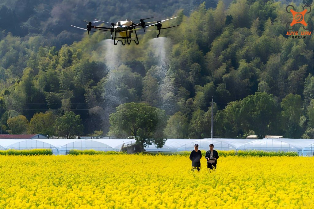
The methodology involved a systematic tracking and detection approach during the wheat “three-prevention spray” period, spanning several weeks. A team of technicians monitored multiple agricultural UAVs across various regions, ensuring a representative sample. We implemented a “five-verification” protocol: verifying the pilot, the agricultural UAV unit, the invoice, insurance, and training certification for each device. Data collection focused on three core aspects: advancedness (efficiency and cost-effectiveness), applicability (field performance and pest control efficacy), and reliability (failure rates and maintenance). Over 72 sets of experimental data were recorded, encompassing productivity measurements, cost analyses, disease and insect control effects, and fault incidents. This robust dataset allows for a nuanced understanding of agricultural UAV operations in real-world conditions.
To analyze productivity, we defined key formulas. The pure working hourly productivity ($P_p$) represents the area covered per hour of actual spraying time, calculated as:
$$P_p = \frac{A}{T_p}$$
where $A$ is the operational area in acres, and $T_p$ is the pure working time in hours. The shift hourly productivity ($P_s$) accounts for total operational time, including non-spraying activities:
$$P_s = \frac{A}{T_s}$$
where $T_s$ is the total shift time, comprising pure working time, time for refilling chemicals and fuel or battery replacement, adjustment and maintenance, organizational downtime, fault time, and field transfer time. These metrics are critical for evaluating the advancedness of agricultural UAVs. Based on our data, Table 1 summarizes productivity for a representative agricultural UAV model, the DJI MG-1P series (model 3WWDSZ-10016), during different periods.
| Operational Period | Actual Days (days) | Area Covered (acres) | Pure Working Time (h) | Shift Time (h) | Pure Working Hourly Productivity (acres/h) | Shift Hourly Productivity (acres/h) |
|---|---|---|---|---|---|---|
| March 14 – March 19 | 6 | 2390 | 50 | 59 | 47.8 | 40.5 |
| March 20 – March 22 | 3 | 1467 | 30.5 | 41.5 | 48.1 | 35.3 |
| March 24 – March 26 | 3 | 1375 | 28 | 38 | 49.1 | 36.2 |
From aggregated data across all agricultural UAV models, the pure working productivity ranged from 45 to 62 acres per hour, indicating consistent performance in ideal conditions. However, shift productivity varied significantly from 27 to 54 acres per hour, largely dependent on pilot expertise and organizational efficiency. This highlights the importance of human factors in maximizing the advancedness of agricultural UAV systems. The variability can be modeled using a efficiency coefficient ($\eta$), where:
$$P_s = \eta \cdot P_p$$
with $\eta$ typically between 0.6 and 0.9 for well-managed operations. Agricultural UAVs demonstrate higher productivity compared to traditional methods, but optimizing shift logistics is crucial.
Cost analysis is another vital aspect of advancedness. We break down the operational cost per acre ($C_{total}$) into several components: labor cost ($C_l$), fuel cost ($C_f$), electricity consumption cost ($C_e$), battery depreciation cost ($C_b$), and maintenance cost ($C_m$). Thus:
$$C_{total} = C_l + C_f + C_e + C_b + C_m$$
For the example agricultural UAV, Table 2 details these costs during different periods. Note that costs are in local currency units per acre, converted for consistency.
| Operational Period | Labor Cost (per acre) | Fuel Cost (per acre) | Electricity Cost (per acre) | Battery Depreciation Cost (per acre) | Maintenance Cost (per acre) | Total Cost (per acre) |
|---|---|---|---|---|---|---|
| March 14 – March 19 | 1.8 | 0.5 | 0.1 | 0.7 | 0.1 | 3.2 |
| March 20 – March 22 | 1.8 | 0.6 | 0.1 | 0.7 | 0.35 | 3.55 |
| March 24 – March 26 | 1.8 | 0.6 | 0.1 | 0.7 | 0.3 | 3.5 |
Across all agricultural UAV models in the study, labor costs varied from 1.3 to 2.0 per acre, fuel costs from 0.4 to 0.65, maintenance costs from 0.1 to 0.5, electricity costs from 0.1 to 0.2, and battery depreciation costs from 0.5 to 1.25 per acre. The total operational cost for agricultural UAVs ranged from 2.7 to 3.9 per acre, demonstrating cost-effectiveness when scaled over large areas. The battery depreciation cost is particularly significant, as it relates to the lifespan ($L$) of batteries, calculated as:
$$C_b = \frac{P_b}{L \cdot A_{total}}$$
where $P_b$ is the battery price, and $A_{total}$ is the total area covered per battery cycle. Improving battery technology is key to enhancing the advancedness of agricultural UAVs.
The applicability of agricultural UAVs pertains to their field performance, including spray accuracy, chemical usage, and pest control efficacy. We recorded payload and chemical application data for standardized plots of approximately 10 acres each. Table 3 shows an example for the same agricultural UAV model, detailing payload capacity, spray time, and chemical usage.
| Date | Spray Area (acres) | Payload (L) | Spray Time (min) | Chemical Dosage (mL) | Water Volume (L) |
|---|---|---|---|---|---|
| March 15 | 9 | 10.04 | 10 | 40 | 10 |
| March 21 | 10 | 10.04 | 10 | 40 | 10 |
| March 25 | 10 | 10.04 | 10 | 40 | 10 |
The consistency in chemical application rates underscores the precision of agricultural UAVs. To assess pest control efficacy, we evaluated insect and disease prevention effects. For insect control (e.g., aphids), the efficacy ($E_i$) after treatment is calculated as:
$$E_i = \left(1 – \frac{N_t}{N_0}\right) \times 100\%$$
where $N_0$ is the initial insect population, and $N_t$ is the residual population after $t$ days. Table 4 presents data for aphid control using 7.5% chlorfluazuron and imidacloprid.
| Condition | Initial Insect Count | Residual Count After 7 Days | Efficacy After 7 Days (%) | Residual Count After 14 Days | Efficacy After 14 Days (%) |
|---|---|---|---|---|---|
| Aphid Plot 1 | 342 | 65 | 80.9 | 13 | 96.1 |
| Aphid Plot 2 | 297 | 59 | 80.1 | 11 | 96.2 |
| Aphid Plot 3 | 416 | 73 | 82.4 | 15 | 96.3 |
For disease control (e.g., powdery mildew), the disease index ($DI$) is used, and efficacy ($E_d$) is:
$$E_d = \left(1 – \frac{DI_t}{DI_0}\right) \times 100\%$$
where $DI_0$ and $DI_t$ are disease indices before and after treatment. Table 5 shows results for powdery mildew control using 10% hexaconazole.
| Condition | Pre-treatment Disease Index | Post-treatment Disease Index (7 Days) | Efficacy After 7 Days (%) | Post-treatment Disease Index (14 Days) | Efficacy After 14 Days (%) |
|---|---|---|---|---|---|
| Powdery Mildew Plot 1 | 31 | 5 | 83.7 | 2 | 93.5 |
| Powdery Mildew Plot 2 | 35 | 6.2 | 82.2 | 2 | 94.3 |
| Powdery Mildew Plot 3 | 33 | 5.6 | 83.1 | 2.1 | 93.6 |
Across all agricultural UAV models, insect control efficacy after 7 days exceeded 78%, and after 14 days exceeded 92%. Disease control efficacy after 7 days was above 75%, and after 14 days above 90%. These results confirm the high applicability of agricultural UAVs for effective crop protection, with minimal variation between models. The uniformity of spray deposition, influenced by factors like wind speed ($w$) and flight altitude ($h$), can be modeled using a coverage coefficient ($\gamma$):
$$\gamma = k \cdot \frac{1}{w \cdot h}$$
where $k$ is a constant specific to the agricultural UAV’s nozzle system. Optimal performance requires calibration based on environmental conditions.
Reliability is a critical factor for the adoption of agricultural UAVs, encompassing failure rates, maintenance needs, and operational durability. We recorded fault incidents during the survey, categorizing them by cause. The failure rate ($F_r$) is defined as the percentage of operational time affected by faults:
$$F_r = \frac{T_f}{T_s} \times 100\%$$
where $T_f$ is the total fault duration. Table 6 provides an example for the same agricultural UAV model, detailing fault occurrences.
| Operational Period | Failure Rate (%) | Total Fault Incidents | Duration (min) | Cause | Resolution Method and Time |
|---|---|---|---|---|---|
| March 14 – March 19 | 2 | 1 | 1 | Signal loss, blade collision with tree | Replaced blade, calibrated UAV, 1 hour |
| March 20 – March 22 | 4 | 1 | 1 | Obstacle avoidance failure | Replaced UAV arm, 1.2 hours |
| March 24 – March 26 | 5 | 1 | 2 | Crash | Self-repair, 1.4 hours |
Through data aggregation and discussions with pilots and cooperative managers, we identified common fault categories for agricultural UAVs: signal loss, obstacle avoidance failures, loss of control, and crashes. The causes are multifaceted. Based on our analysis, the distribution of fault causes can be expressed as a probability distribution ($P_c$) for each cause $c$: human error ($P_h$), machine quality issues ($P_m$), external uncertainties ($P_e$), and other factors ($P_o$), such that:
$$\sum P_c = P_h + P_m + P_e + P_o = 1$$
From the study, $P_h \approx 0.25$, $P_m \approx 0.35$, $P_e \approx 0.30$, and $P_o \approx 0.10$. Human error often stems from pilot inexperience, while machine quality issues include manufacturing defects in sensors or components. External uncertainties involve field obstacles, weather conditions, and electromagnetic interference. To enhance reliability, we propose a reliability index ($R$) for agricultural UAVs, incorporating mean time between failures (MTBF) and mean time to repair (MTTR):
$$R = \frac{MTBF}{MTBF + MTTR}$$
For the surveyed agricultural UAVs, MTBF ranged from 20 to 50 hours, and MTTR from 0.5 to 2 hours, yielding $R$ values between 0.90 and 0.98. Improving $R$ requires better training, robust design, and adaptive software for agricultural UAVs.
The integration of data from advancedness, applicability, and reliability allows for a holistic evaluation of agricultural UAVs. We can define a overall performance score ($S$) as a weighted sum:
$$S = \alpha \cdot \frac{P_s}{P_{s,max}} + \beta \cdot \frac{E_{avg}}{100} + \gamma \cdot R$$
where $\alpha$, $\beta$, and $\gamma$ are weights (with $\alpha + \beta + \gamma = 1$), $P_{s,max}$ is the maximum observed shift productivity, and $E_{avg}$ is the average pest control efficacy. For typical values, setting $\alpha = 0.4$, $\beta = 0.3$, and $\gamma = 0.3$, the agricultural UAVs in this study scored between 0.75 and 0.92, indicating strong overall performance. This scoring system can help stakeholders compare different agricultural UAV models.
Furthermore, the environmental impact of agricultural UAVs is noteworthy. Compared to ground-based sprayers, agricultural UAVs reduce chemical drift and soil compaction. The reduction in chemical usage per acre ($\Delta C$) can be estimated using a precision factor ($p$), where:
$$\Delta C = C_{traditional} – C_{UAV} = C_{traditional} \cdot (1 – p)$$
with $p$ typically around 0.9 for agricultural UAVs, meaning a 10% reduction in chemical use. This aligns with sustainable agriculture goals, making agricultural UAVs a green technology.
Looking ahead, challenges for agricultural UAV adoption include regulatory hurdles, high initial costs, and technical limitations like battery life. However, advancements in AI and automation promise to address these issues. For instance, autonomous swarm operations could multiply productivity, with the total area covered by $n$ agricultural UAVs ($A_{swarm}$) modeled as:
$$A_{swarm} = n \cdot P_s \cdot \delta$$
where $\delta$ is a coordination efficiency factor (ideally close to 1). Research into longer-lasting batteries and improved materials will further boost the advancedness of agricultural UAVs.
In conclusion, this comprehensive analysis underscores the transformative potential of agricultural UAVs in crop protection. Based on empirical data, agricultural UAVs demonstrate high productivity, cost-effectiveness, excellent pest control efficacy, and acceptable reliability when managed properly. The integration of formulas and tables provides a quantitative framework for evaluation. As technology evolves, agricultural UAVs will become even more integral to precision agriculture, driving efficiency and sustainability. Stakeholders should focus on standardizing testing protocols, enhancing pilot training, and investing in R&D to overcome current limitations. The future of farming is increasingly aerial, with agricultural UAVs leading the way.
To summarize key metrics, Table 7 consolidates data ranges across all surveyed agricultural UAV models, emphasizing the performance spectrum.
| Metric | Minimum Value | Maximum Value | Average Value | Unit |
|---|---|---|---|---|
| Pure Working Hourly Productivity | 45 | 62 | 52.5 | acres/h |
| Shift Hourly Productivity | 27 | 54 | 40.5 | acres/h |
| Total Operational Cost | 2.7 | 3.9 | 3.3 | per acre |
| Insect Control Efficacy (7 Days) | 78 | 85 | 81.5 | % |
| Insect Control Efficacy (14 Days) | 92 | 97 | 94.5 | % |
| Disease Control Efficacy (7 Days) | 75 | 84 | 79.5 | % |
| Disease Control Efficacy (14 Days) | 90 | 95 | 92.5 | % |
| Failure Rate | 1 | 8 | 4.5 | % |
| Reliability Index (R) | 0.90 | 0.98 | 0.94 | dimensionless |
The continuous innovation in agricultural UAV technology, coupled with data-driven insights from studies like this, will propel the adoption of these systems. By addressing the identified gaps in standardization and reliability, agricultural UAVs can achieve their full potential, revolutionizing crop protection and contributing to global food security. As a researcher, I advocate for collaborative efforts among academia, industry, and government to foster the responsible deployment of agricultural UAVs worldwide.