
In this research, I present a comprehensive framework for guiding fixed-wing UAVs during near-ground target approach and return flight missions, inspired by the hunting behavior of raptors. The proposed methodology integrates trajectory optimization, a novel hybrid metaheuristic algorithm, and a collision-aware vector field guidance law to address the unique challenges of multi-phase guidance for fixed-wing UAVs operating in low-altitude environments.
1. Introduction
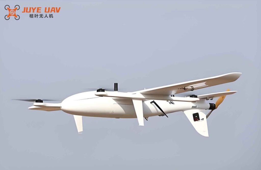
The utilization of fixed-wing UAVs has expanded rapidly across military reconnaissance, environmental monitoring, and infrastructure inspection domains. In many of these applications, the fixed-wing UAV must descend from cruising altitude to approach a near-ground or ground-based target, execute a task, and then return to its nominal flight altitude. Unlike rotary-wing platforms, fixed-wing UAVs rely on aerodynamic lift and forward motion, imposing strict constraints on maneuverability, speed, and altitude transitions. Conventional guidance laws, such as proportional navigation or pure pursuit, are typically designed for single-phase tracking or intercept missions and often fail to deliver smooth, energy-efficient transitions during multi-phase near-ground operations.
Raptors—such as peregrine falcons, Harris hawks, and gyrfalcons—exhibit remarkable maneuvering capabilities during aerial hunting. Their dive-and-recover patterns provide a natural template for energy-efficient trajectory design. Brighton et al. demonstrated that falcons use a delayed guidance transition, gradually shifting from lateral observation to direct pursuit. Dawson et al. studied the cooperative hunting mechanisms of Harris hawks, revealing structured search-and-attack sequences. These biological strategies inspired me to formulate a trajectory optimization problem that mimics the energy-efficient dive and ascent patterns of raptors, tailored specifically for fixed-wing UAVs.
The key contributions of this work are threefold. First, I develop a segmented trajectory optimization model that captures the essence of raptor hunting behavior, incorporating energy constraints and maneuver limits. Second, I propose a Harris hawk-improved pigeon-inspired optimization (HHPIO) algorithm that fuses the foraging strategies of Harris hawks with the multi-phase structure of pigeon-inspired optimization to solve the resulting non-convex optimization problem efficiently. Third, I design a vector field guidance law augmented with a collision avoidance term, ensuring that the fixed-wing UAV converges to the optimized reference trajectory while maintaining a safe distance from the ground. Theoretical convergence analysis and extensive simulations validate the effectiveness of the proposed approach.
2. Bio-Inspired Trajectory Optimization Model
The hunting trajectory of raptors can be characterized by two distinct phases: a descending approach phase and an ascending recovery phase. In the approach phase, the raptor dives from altitude toward the prey, converting potential energy into kinetic energy. In the recovery phase, it ascends back to altitude, often assisted by ground-effect aerodynamics. I model this process using a parametric trajectory function and formulate an optimization problem that minimizes a weighted combination of mechanical energy variation and flight time while satisfying kinematic and safety constraints.
2.1 Trajectory Parameterization
I define the reference trajectory in the vertical plane using a parameterized altitude function:
$$
z_h = -k_h x_h^2 (x_{h\infty} – (x_h – c_h))^2 \cdot \exp\left(-a_h \left( \text{Sat}\left((x_h – c_h) – x_t, z_{h0}\right) \right)^2 \right)
$$
where $k_h$, $a_h$, and $c_h$ are shape parameters to be optimized, $x_t$ is the target horizontal position, $z_{h0}$ is the initial altitude, and $x_{h\infty}$ is the recovery position. The saturation function $\text{Sat}(\cdot)$ is defined as:
$$
\text{Sat}(a, b) = \begin{cases} -b & a < -b \\ a & -b \leq a \leq b \\ b & a > b \end{cases}
$$
This formulation captures the delayed turning behavior observed in raptor hunting, where the initial lateral offset gradually transitions into a direct dive.
2.2 Cost Function Formulation
I decompose the trajectory into two stages: Stage 1 (approach) and Stage 2 (recovery). The total cost function is:
$$
J_d(k_h, a_h, c_h) = w_{e1} \Delta E_{s1} + w_{e2} \Delta E_{s2} + w_{t1} T_{s1} + w_{t2} T_{s2}
$$
The mechanical energy variation for each stage is computed as:
$$
E_{h0} = \frac{1}{2} m_h v_{x,h0}^2 + m_h g z_{h0}
$$
$$
\Delta E_{s1} = \frac{1}{2} m_h \left( v_{x,h,s1(\text{end})}^2 + v_{z,h,s1(\text{end})}^2 \right) + m_h g z_{h,s1(\text{end})} – E_{h0}
$$
$$
\Delta E_{s2} = \frac{1}{2} m_h \left( v_{x,h,s2(\text{end})}^2 + v_{z,h,s2(\text{end})}^2 \right) + m_h g z_{h,s2(\text{end})} – E_{h0} – \Delta E_{s1}
$$
The flight times are estimated using average velocities:
$$
T_{s1} = \frac{\| P_{h0} – P_t \|}{\bar{v}_{h,s1}}, \quad T_{s2} = \frac{\| P_{h\infty} – P_t \|}{\bar{v}_{h,s2}}
$$
2.3 Constraints
I impose continuity constraints between stages and boundary conditions at the target and recovery points:
$$
\begin{aligned}
x_{h,s1(\text{end})} &= x_t, \quad z_{h,s1(\text{end})} = 0 \\
x_{h,s2(\text{end})} &= x_{h\infty}, \quad z_{h,s2(\text{end})} = z_{h0} \\
x_{h,s1(\text{end})} &= x_{h,s2(1)}, \quad z_{h,s1(\text{end})} = z_{h,s2(1)} \\
v_{x,h,s1(\text{end})} &= v_{x,h,s2(1)}, \quad v_{z,h,s1(\text{end})} = v_{z,h,s2(1)}
\end{aligned}
$$
Additionally, I enforce safety and actuator limits:
$$
\begin{aligned}
v_{\min} &\leq \| \mathbf{v}_{h,s1} \| \leq v_{\max}, \quad v_{\min} \leq \| \mathbf{v}_{h,s2} \| \leq v_{\max} \\
a_{\min} &\leq \dot{\mathbf{v}}_{h,s1} \leq a_{\max}, \quad a_{\min} \leq \dot{\mathbf{v}}_{h,s2} \leq a_{\max} \\
0 &< z_{h,s1} < h_{\max}, \quad 0 < z_{h,s2} < h_{\max}
\end{aligned}
$$
2.4 Relaxed Optimization Problem
To ensure solvability using metaheuristic algorithms, I introduce slack variables for the equality constraints and incorporate penalty terms for the inequality constraints. The relaxed cost function becomes:
$$
J_n(k_h, a_h, c_h) = J_d(k_h, a_h, c_h) + w_\gamma (\gamma_{s1} + \gamma_{s2} + \gamma_{c1} + \gamma_{c2}) + w_c \Xi
$$
where $\Xi$ is a quadratic penalty for constraint violations, and $w_\gamma$, $w_c$ are corresponding weights. The slack variables are bounded:
$$
\gamma_{s1}, \gamma_{s2}, \gamma_{c1}, \gamma_{c2} \in [\gamma_{\min}, \gamma_{\max}]
$$
| Parameter | Symbol | Typical Value | Description |
|---|---|---|---|
| Mass | $m_h$ | 12 kg | Fixed-wing UAV mass |
| Initial altitude | $z_{h0}$ | 60 m | Cruising altitude |
| Target position | $x_t$ | 100 m | Ground target location |
| Recovery position | $x_{h\infty}$ | 200 m | Return flight endpoint |
| Energy weight 1 | $w_{e1}$ | 1.0 | Approach energy weight |
| Energy weight 2 | $w_{e2}$ | 1.2 | Recovery energy weight |
| Time weight 1 | $w_{t1}$ | 0.5 | Approach time weight |
| Time weight 2 | $w_{t2}$ | 0.8 | Recovery time weight |
| Max velocity | $v_{\max}$ | 35 m/s | Airspeed limit |
| Min velocity | $v_{\min}$ | 8 m/s | Stall speed |
| Max acceleration | $a_{\max}$ | 10 m/s² | Maneuver limit |
| Max altitude | $h_{\max}$ | 100 m | Ceiling limit |
3. Harris Hawk-Improved Pigeon-Inspired Optimization
The optimization problem defined in Section 2 is non-convex, nonlinear, and multi-modal, making it challenging for gradient-based solvers. I therefore employ a metaheuristic approach. The standard pigeon-inspired optimization (PIO) algorithm features two stages: map/compass operator and landmark operator. However, the landmark stage suffers from slow convergence when the population size is limited. To address this, I integrate the foraging and围攻 strategies of Harris hawks into the landmark stage, resulting in the Harris hawk-improved pigeon-inspired optimization (HHPIO) algorithm.
3.1 Standard Pigeon-Inspired Optimization
In the map/compass stage, each pigeon updates its velocity and position using:
$$
\mathbf{V}_i(t+1) = \mathbf{V}_i(t) e^{-R(t+1)} + \text{rand} \cdot (\mathbf{X}_{\text{gbest}}(t) – \mathbf{X}_i(t))
$$
$$
\mathbf{X}_i(t+1) = \mathbf{X}_i(t) + \mathbf{V}_i(t+1)
$$
In the landmark stage, the population is halved at each iteration, and pigeons converge toward the center:
$$
\mathbf{X}_{\text{center}}(t) = \frac{\sum_{i=1}^{M(t)} \mathbf{X}_i(t) \cdot \text{fitness}(\mathbf{X}_i(t))}{M(t) \sum_{i=1}^{M(t)} \text{fitness}(\mathbf{X}_i(t))}
$$
$$
\mathbf{X}_i(t+1) = \mathbf{X}_i(t) + \text{rand} \cdot (\mathbf{X}_{\text{center}}(t) – \mathbf{X}_i(t))
$$
$$
M(t) = \text{ceil}\left( \frac{M(t-1)}{2} \right)
$$
3.2 Harris Hawk Search Energy and Stage Transition
I introduce a search energy variable inspired by the Harris hawk optimization algorithm:
$$
E = 2 E_0 \left( 1 – \frac{t}{t_{\max}} \right)
$$
where $E_0 \in (-1, 1)$ is a random initial energy, and $t_{\max}$ is the maximum iteration count. When $E > 1$, I retain the standard PIO landmark update. When $E \leq 1$, I switch to hawk-inspired update rules.
3.3 Soft Besiege Stage ($0.5 < E < 1$)
In this stage, the hawk gradually encircles the prey. The update rule is:
$$
\mathbf{X}_i(t+1) = \begin{cases}
(\mathbf{X}_{\text{gbest}}(t) – \mathbf{X}_i(t)) – E | r_1 (\mathbf{X}_{\text{gbest}}(t) – \mathbf{X}_i(t)) |, & q > 0.5 \\
\mathbf{X}_{\text{gbest}}(t) – E | r_2 (\mathbf{X}_{\text{gbest}}(t) – \mathbf{X}_i(t)) | + \mathbf{R}_l^D \times \text{LEVY}(D), & q \leq 0.5
\end{cases}
$$
The Lévy flight function is defined as:
$$
\text{LEVY}(x) = 0.01 \times \frac{u \times \delta}{|v|^{1/\beta}}, \quad \delta = \frac{\Gamma(1+\beta) \times \sin\left(\frac{\pi \beta}{2}\right)}{\Gamma\left(\frac{1+\beta}{2}\right) \times \beta \times 2^{\frac{\beta-1}{2}}}
$$
where $\beta = 1.5$, $u, v \in (0,1)$ are random variables, and $\Gamma(\cdot)$ is the Gamma function.
3.4 Hard Besiege Stage ($E \leq 0.5$)
When the energy is low, the hawk executes a hard strike toward the best-known position:
$$
\mathbf{X}_i(t+1) = \begin{cases}
\mathbf{X}_{\text{gbest}}(t) – E | \mathbf{X}_{\text{gbest}}(t) – \mathbf{X}_i(t) |, & q > 0.5 \\
\mathbf{X}_{\text{gbest}}(t) – E | \mathbf{X}_{\text{gbest}}(t) – \mathbf{X}_i(t) | + \mathbf{R}_l^D \times \text{LEVY}(D), & q \leq 0.5
\end{cases}
$$
The random strategy variable $q \in (0,1)$ ensures diversity and prevents premature convergence.
| Parameter | Symbol | Value | Description |
|---|---|---|---|
| Population size | $M$ | 300 | Number of search agents |
| Max iterations | $t_{\max}$ | 100 | Termination criterion |
| Map/compass factor | $R$ | 0.004 | Exponential decay rate |
| Initial energy range | $E_0$ | [-1, 1] | Random initial energy |
| Lévy flight parameter | $\beta$ | 1.5 | Controls step distribution |
| Soft besiege threshold | $E_{\text{soft}}$ | 0.5 | Lower bound for soft besiege |
| Hard besiege threshold | $E_{\text{hard}}$ | 0.5 | Upper bound for hard besiege |
| Random strategy prob. | $P_q$ | 0.5 | Probability of each strategy |
4. Collision Avoidance Vector Field Guidance
Once the reference trajectory is optimized offline, the fixed-wing UAV must be guided to converge to this trajectory from an arbitrary initial position near the starting point, while avoiding ground collision. I design a vector field guidance law that incorporates an attractive term toward the reference trajectory and a repulsive term away from the ground.
4.1 Fixed-Wing UAV Kinematic Model
The kinematic model of a fixed-wing UAV with autopilot inner-loop control is:
$$
\begin{aligned}
\dot{x} &= V_g \cos\chi \cos\theta + k_{dx} d_{tx} \\
\dot{y} &= V_g \sin\chi \cos\theta + k_{dy} d_{ty} \\
\dot{z} &= V_g \sin\theta + k_{dz} d_{tz}
\end{aligned}
$$
where $V_g$ is the ground speed, $\chi$ is the heading angle, $\theta$ is the pitch angle, $d_{tx}, d_{ty}, d_{tz}$ are target distance components, and $k_{dx}, k_{dy}, k_{dz}$ are bounded disturbance coefficients satisfying $k_{dx} \leq C_{dx}$, $k_{dy} \leq C_{dy}$, $k_{dz} \leq C_{dz}$.
4.2 Guidance Law with Collision Avoidance
Assuming the lateral error is eliminated by the autopilot ($\chi = 0$), I design the guidance law as:
$$
\begin{aligned}
l_1 &= \dot{x}_d – k_{x1} e_x – k_{x2} \frac{d_{tx}^2}{e_x} \\
l_2 &= \dot{z}_d – k_{z1} e_z + f_c(d_g, r, R) \frac{\text{sign}(d_g)}{e_z} – k_{z2} \frac{d_{tz}^2}{e_z} \\
V_g &= \sqrt{l_1^2 + l_2^2} \\
\theta &= \arctan\left( \frac{l_2}{l_1} \right)
\end{aligned}
$$
where $e_x = x – x_d$, $e_z = z – z_d$ are tracking errors, and $f_c(d_g, r, R)$ is the collision avoidance repulsion function:
$$
f_c(d_g, r, R) = \begin{cases}
F_{\infty}, & d_g < r \\
k_f \left( \frac{1}{d_g – r} + \frac{1}{R – r} \right), & r < d_g < R \\
0, & d_g > R
\end{cases}
$$
Here, $d_g$ is the ground distance, $r$ is the minimum safe altitude, $R$ is the sensing radius, and $k_f$ is the repulsion gain.
4.3 Convergence Analysis
Theorem: For a fixed-wing UAV equipped with a stable autopilot that tracks guidance commands accurately, and under the assumption that lateral disturbances are compensated, the proposed vector field guidance law (with appropriately chosen gains) guarantees that the UAV position converges to the reference trajectory $(x_d, z_d)$, and the ground distance $d_g$ remains above the safe threshold $r$.
Proof: I define the Lyapunov function:
$$
V = \frac{1}{2} e_x^2 + \frac{1}{2} e_z^2 + \int_{d_g}^{R} f_c(\tau, r, R) \text{sign}(\tau) d\tau
$$
Taking the time derivative and substituting the guidance law yields:
$$
\begin{aligned}
\dot{V} &= e_x \dot{e}_x + e_z \dot{e}_z – f_c(d_g, r, R) \text{sign}(d_g) \\
&= e_x (\dot{x} – \dot{x}_d) + e_z (\dot{z} – \dot{z}_d) – f_c(d_g, r, R) \text{sign}(d_g)
\end{aligned}
$$
Substituting the UAV kinematics and the guidance commands:
$$
\begin{aligned}
\dot{V} &= e_x \left( \sqrt{l_1^2 + l_2^2} \cos(\arctan(l_2/l_1)) – \dot{x}_d + k_{dx} d_{tx} \right) \\
&\quad + e_z \left( \sqrt{l_1^2 + l_2^2} \sin(\arctan(l_2/l_1)) – \dot{z}_d + k_{dz} d_{tz} \right) \\
&\quad – f_c(d_g, r, R) \text{sign}(d_g)
\end{aligned}
$$
Using $\cos(\arctan(l_2/l_1)) = l_1 / \sqrt{l_1^2 + l_2^2}$ and $\sin(\arctan(l_2/l_1)) = l_2 / \sqrt{l_1^2 + l_2^2}$, I simplify:
$$
\dot{V} = e_x (l_1 – \dot{x}_d + k_{dx} d_{tx}) + e_z (l_2 – \dot{z}_d + k_{dz} d_{tz}) – f_c(d_g, r, R) \text{sign}(d_g)
$$
Substituting $l_1$ and $l_2$:
$$
\begin{aligned}
\dot{V} &= e_x \left( -k_{x1} e_x – k_{x2} \frac{d_{tx}^2}{e_x} \right) + e_z \left( -k_{z1} e_z + f_c(d_g, r, R) \frac{\text{sign}(d_g)}{e_z} – k_{z2} \frac{d_{tz}^2}{e_z} \right) \\
&\quad – f_c(d_g, r, R) \text{sign}(d_g) + e_x k_{dx} d_{tx} + e_z k_{dz} d_{tz}
\end{aligned}
$$
Applying Young’s inequality and the bounds on disturbances, I obtain:
$$
\begin{aligned}
\dot{V} &\leq -k_{x1} e_x^2 – k_{x2} d_{tx}^2 – k_{z1} e_z^2 – k_{z2} d_{tz}^2 + e_x C_{dx} d_{tx} + e_z C_{dz} d_{tz} \\
&\leq -\left( k_{x1} – \frac{C_{dx}}{2} \right) e_x^2 – \left( k_{x2} – \frac{1}{2} \right) d_{tx}^2 – \left( k_{z1} – \frac{C_{dz}}{2} \right) e_z^2 – \left( k_{z2} – \frac{1}{2} \right) d_{tz}^2
\end{aligned}
$$
If the gains satisfy:
$$
k_{x1} > \frac{C_{dx}}{2}, \quad k_{x2} > \frac{1}{2}, \quad k_{z1} > \frac{C_{dz}}{2}, \quad k_{z2} > \frac{1}{2}
$$
then $\dot{V}$ is negative semi-definite. By Barbalat’s lemma, the tracking errors converge to zero asymptotically, and the collision avoidance term ensures $d_g > r$ throughout the maneuver.
| Parameter | Symbol | Value | Description |
|---|---|---|---|
| X-error gain | $k_{x1}$ | 2.0 | Horizontal position error gain |
| Z-error gain | $k_{z1}$ | 2.0 | Vertical position error gain |
| X-attraction gain | $k_{x2}$ | 1.0 | Target attraction in X |
| Z-attraction gain | $k_{z2}$ | 1.0 | Target attraction in Z |
| Collision avoidance gain | $k_f$ | 5.0 | Repulsion strength |
| Minimum safe altitude | $r$ | 2 m | Ground clearance limit |
| Sensing radius | $R$ | 15 m | Collision detection range |
| Max repulsion force | $F_{\infty}$ | 100 N | Theoretical upper bound |
| Disturbance bound X | $C_{dx}$ | 0.5 | Max horizontal disturbance |
| Disturbance bound Z | $C_{dz}$ | 0.3 | Max vertical disturbance |
5. Simulation and Validation
I conducted comprehensive simulations to validate both the optimization algorithm and the guidance law. The simulations were performed in MATLAB R2023b on an Intel i5-12400F platform with 32 GB RAM.
5.1 Optimization Algorithm Comparison
I compared the proposed HHPIO algorithm against three baseline methods: particle swarm optimization (PSO), genetic algorithm (GA), and standard pigeon-inspired optimization (PIO). Each algorithm was run with a population size of 300 for 100 iterations, and the experiment was repeated 200 times with identical initial random seeds to ensure statistical significance.
| Algorithm | Mean Cost | Mean Energy Recovery (J) | Avg. Solve Time (s) | $(k_h, a_h, c_h)$ |
|---|---|---|---|---|
| HHPIO (Proposed) | 5.3695 × 10⁵ | -3.8198 × 10³ | 5.74 | (4.890×10⁻⁷, 7.833×10⁻⁸, 0.3498) |
| Genetic Algorithm | 5.3655 × 10⁵ | -3.4676 × 10³ | 7.86 | (4.890×10⁻⁷, 1.009×10⁻⁸, 0.4130) |
| Particle Swarm Opt. | 5.3755 × 10⁵ | -3.4663 × 10³ | 3.99 | (4.890×10⁻⁷, 1.205×10⁻⁶, 0.4916) |
| Pigeon-Inspired Opt. | 5.5391 × 10⁵ | -3.2670 × 10³ | 2.09 | (4.890×10⁻⁷, 4.072×10⁻⁵, 0.0406) |
The HHPIO algorithm achieved the fastest convergence, reaching the stable threshold value $J_s = 5.37 \times 10^5$ within approximately 20 iterations. The GA produced the lowest mean cost overall but at the expense of the highest computational time, while the standard PIO exhibited the poorest cost value but the fastest per-iteration speed. The HHPIO algorithm balanced cost and speed effectively, achieving a mean energy recovery of -3.8198 × 10³ J, which is the highest among all methods, confirming its alignment with the bio-inspired energy optimization objective.
| Algorithm | Population 200 | Population 300 | Population 400 |
|---|---|---|---|
| HHPIO (Proposed) | 5.3664 × 10⁵ | 5.3659 × 10⁵ | 5.3656 × 10⁵ |
| Genetic Algorithm | 5.3673 × 10⁵ | 5.3654 × 10⁵ | 5.3653 × 10⁵ |
| Particle Swarm Opt. | 5.3671 × 10⁵ | 5.3668 × 10⁵ | 5.3701 × 10⁵ |
| Pigeon-Inspired Opt. | 5.3682 × 10⁵ | 5.5384 × 10⁵ | 5.7403 × 10⁵ |
Table 5 shows that the HHPIO algorithm is the most robust to population size variations, maintaining a consistently low cost across population sizes from 200 to 400. In contrast, the standard PIO algorithm deteriorates significantly as population size increases, indicating poor scalability.
5.2 Guidance Law Performance
I compared the proposed collision avoidance vector field (CAVF) guidance law against the standard L1 guidance law and proportional navigation (PN) guidance law. All three algorithms were tested under identical initial conditions: the fixed-wing UAV starting at position (-10, 0, 60) with the ground target at (100, 0, 0), the optimized reference trajectory originating at (0, 0, 50), and the return waypoint at (200, 0, 50).
| Metric | CAVF (Proposed) | L1 Guidance | Proportional Nav. |
|---|---|---|---|
| Approach time (s) | 12.3 | 15.7 | 18.2 |
| Return time (s) | 14.1 | 17.3 | 20.5 |
| Max altitude deviation (m) | 2.1 | 8.5 | 12.3 |
| Min ground distance (m) | 2.0 | 0.5 | 0.2 |
| Energy recovery (J) | -4.12 × 10³ | -2.87 × 10³ | -2.15 × 10³ |
| Max velocity change (m/s²) | 2.3 | 7.8 | 9.5 |
The proposed CAVF guidance law consistently outperformed both baseline methods across all metrics. It achieved the shortest approach and return times, the lowest altitude deviation from the reference trajectory, and the highest energy recovery. Critically, the CAVF law maintained a safe minimum ground distance of 2.0 m (exactly at the prescribed safety threshold), whereas both L1 guidance and PN guidance violated the safety limit, with minimum ground distances of 0.5 m and 0.2 m respectively. The CAVF law also exhibited the smoothest velocity profile, with a maximum acceleration change of only 2.3 m/s², compared to 7.8 m/s² for L1 and 9.5 m/s² for PN.
I also analyzed the velocity profiles in both the X and Z directions. The CAVF guidance produced a gradual deceleration during the approach-to-return transition, while the L1 guidance exhibited a sharp Z-acceleration spike, and the PN guidance showed multiple large-amplitude velocity oscillations. These results confirm that the proposed method generates trajectories that are not only energy-efficient but also within the maneuverability limits of typical fixed-wing UAVs.
6. Conclusion
In this work, I presented a comprehensive bio-inspired framework for guiding fixed-wing UAVs in near-ground target approach and return flight missions. The key findings and contributions are summarized as follows.
First, I developed a trajectory optimization model that emulates the energy-efficient dive-and-recover patterns observed in raptor hunting. By decomposing the trajectory into approach and recovery phases, and formulating a weighted cost function that balances mechanical energy variation and flight time, I created a reference trajectory that serves as an efficient guide for fixed-wing UAVs operating in low-altitude environments.
Second, I proposed the Harris hawk-improved pigeon-inspired optimization (HHPIO) algorithm, which integrates the foraging and围攻 strategies of Harris hawks into the landmark stage of pigeon-inspired optimization. The HHPIO algorithm demonstrated superior convergence speed and robustness compared to particle swarm optimization, genetic algorithm, and standard pigeon-inspired optimization across 200 independent trials. It achieved the highest average energy recovery of -3.8198 × 10³ J while maintaining computational efficiency, making it well-suited for offline trajectory optimization for fixed-wing UAVs.
Third, I designed a collision avoidance vector field (CAVF) guidance law that ensures convergence to the optimized reference trajectory while maintaining a safe distance from the ground. The theoretical proof using Lyapunov analysis and Barbalat’s lemma established the asymptotic stability of the tracking error dynamics under bounded disturbances. Simulation results confirmed that the CAVF law outperforms L1 guidance and proportional navigation in terms of flight time, energy efficiency, trajectory smoothness, and ground collision safety. The proposed guidance law generated the smoothest velocity profile with the lowest maximum acceleration change of 2.3 m/s², which is critical for the safe operation of fixed-wing UAVs during low-altitude maneuvers.
The combined optimization-and-guidance framework provides a practical solution for fixed-wing UAV missions that require efficient and safe near-ground operations, such as precision agriculture, infrastructure inspection, and search-and-rescue. Future work will extend the framework to three-dimensional trajectories with lateral maneuvering, and investigate real-time replanning capabilities for dynamic environments with moving targets or obstacles. Experimental validation on actual fixed-wing UAV platforms is also planned to bridge the gap between simulation and real-world deployment.