
Trajectory planning forms the fundamental bridge between a high-level mission command and the low-level flight control of a quadrotor drone. The primary objective is to generate a feasible path from a start point to a goal point while avoiding obstacles. However, many classic path-finding algorithms, such as A* or Rapidly-exploring Random Trees (RRT), produce paths comprised of straight-line segments connecting waypoints. While these paths are geometrically safe, they are fundamentally unsuitable for direct execution by a quadrotor drone. The sharp corners or “kinks” at the waypoints represent points of discontinuity in the higher-order derivatives of the position. Since the dynamics of a quadrotor drone are intimately linked to these derivatives—specifically, velocity, acceleration, and jerk—following such a path would require instantaneous changes in motor thrust, which is physically impossible. This leads to significant tracking error, excessive energy consumption, and mechanical stress.
The core challenge, therefore, is not just to find a path, but to optimize it into a smooth, dynamically feasible trajectory—a time-parameterized path where the position, and its derivatives, are continuous and respect the physical limits of the vehicle. This process is often termed “trajectory generation” or “path smoothing.” In this article, I will discuss a powerful optimization framework based on Bézier curves and convex optimization that transforms a discrete, jagged path into a smooth, safe, and efficient trajectory for a quadrotor drone.
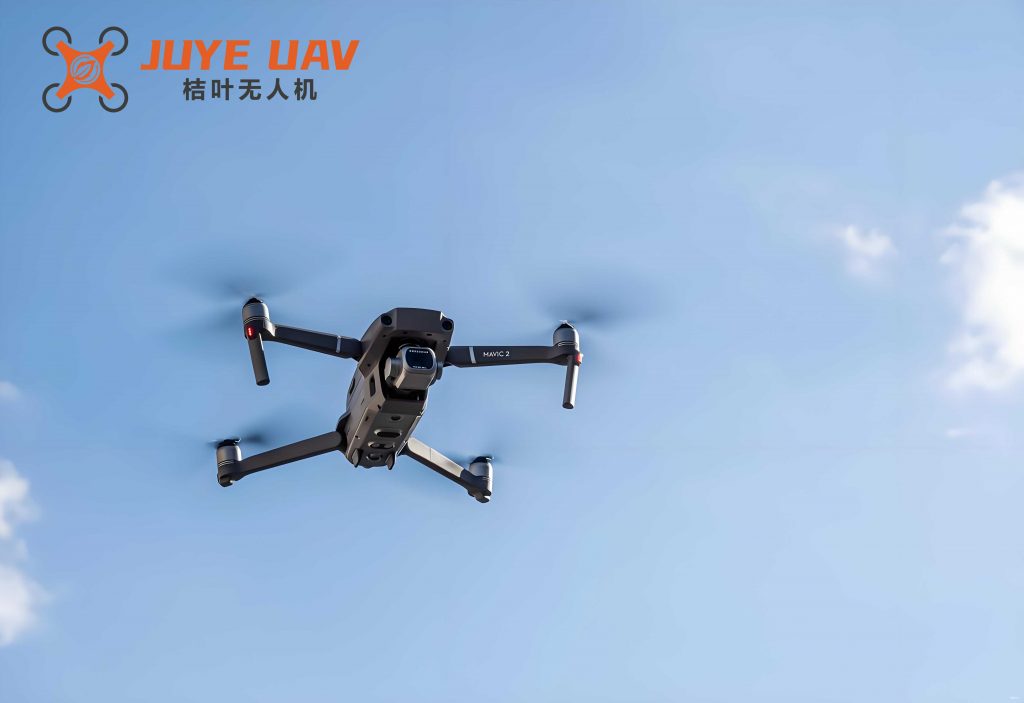
The Dynamics of a Quadrotor Drone and Trajectory Requirements
A quadrotor drone is an underactuated system. It has four control inputs (the rotational speeds of its four motors) but six degrees of freedom (position and orientation in 3D space). Its translational motion is achieved by tilting its body, which reorients the total thrust vector. The relationship between the desired trajectory and the control inputs is complex and involves high-order derivatives. For a typical hierarchical controller, the position controller outputs a desired acceleration. This desired acceleration is then converted into a desired attitude and total thrust for the lower-level attitude controller to track.
Consequently, for the position controller to function correctly and for the resulting commands to be physically achievable, the reference trajectory must be smooth. More formally, we require the trajectory to be differentiable up to at least the fourth order (snap). The reasons are as follows:
- Velocity (1st derivative): Must be continuous to avoid infinite acceleration.
- Acceleration (2nd derivative): Directly related to the net force/thrust on the quadrotor drone. Discontinuities would imply instantaneous force changes.
- Jerk (3rd derivative): Related to the rate of change of force, affecting passenger comfort and actuator effort.
- Snap (4th derivative): Related to the differential thrust required for aggressive attitude changes. Minimizing snap often leads to smoother motor commands.
Thus, a key optimization objective for a quadrotor drone trajectory is to minimize the integral of the squared magnitude of the fourth derivative (snap) or a similar high-order derivative over the flight time.
The Minimum-Snap Trajectory Optimization Problem
A standard approach to creating smooth trajectories is to represent each segment of the path between two waypoints as a polynomial function of time. For a trajectory divided into \(M\) segments, the position in one dimension (e.g., \(x\)) can be written as a piecewise polynomial:
$$f_\mu(t) = \begin{cases}
\sum_{j=0}^{N} p_{1j} (t – T_0)^j & T_0 \leq t \leq T_1\\
\sum_{j=0}^{N} p_{2j} (t – T_1)^j & T_1 \leq t \leq T_2\\
\vdots & \\
\sum_{j=0}^{N} p_{Mj} (t – T_{M-1})^j & T_{M-1} \leq t \leq T_M
\end{cases}$$
where \(\mu \in \{x, y, z\}\), \(p_{ij}\) is the \(j\)-th coefficient of the polynomial for the \(i\)-th segment, and \(T_i\) are the segment endpoint times. The polynomial order \(N\) is chosen to be sufficiently high (e.g., 7th or 9th order) to allow enforcement of boundary conditions on position, velocity, acceleration, and jerk at the waypoints.
The optimization goal is to find the set of polynomial coefficients \(p_{ij}\) that minimize a cost function, typically the integral of squared snap:
$$J = \sum_{\mu \in \{x,y,z\}} \int_{0}^{T} \left( \frac{d^4 f_\mu(t)}{dt^4} \right)^2 dt = \sum_{\mu \in \{x,y,z\}} \int_{0}^{T} (f_\mu^{(4)}(t))^2 dt$$
This cost function can be expanded and written in a quadratic form for each segment. For a single segment of duration \(s_i = T_i – T_{i-1}\), after a time-normalizing substitution \(\tau = (t – T_{i-1})/s_i \in [0,1]\), the cost for dimension \(\mu\) and segment \(i\) becomes:
$$J_i = \int_{0}^{s_i} (f^{(4)}(t))^2 dt = \frac{1}{s_i^7} \mathbf{p}_i^T \mathbf{Q}_i \mathbf{p}_i$$
where \(\mathbf{p}_i\) is the vector of polynomial coefficients for segment \(i\), and \(\mathbf{Q}_i\) is a constant Hessian matrix derived from the integration of the polynomial basis functions. The total cost \(J\) is the sum of these segment costs across all three dimensions.
The optimization is subject to several constraints:
- Waypoint Constraints: The trajectory must pass through specified waypoints at specific times, potentially with specified derivatives (e.g., zero velocity at start and end).
- Continuity Constraints: To ensure smoothness, the derivatives (position, velocity, acceleration, jerk) must be continuous at the junctions between segments.
Both sets of constraints are linear equality constraints on the polynomial coefficients \(\mathbf{p} = [\mathbf{p}_1, \mathbf{p}_2, …, \mathbf{p}_M]^T\). The problem can thus be formulated as a Quadratic Programming (QP) problem:
$$\min_{\mathbf{p}} \mathbf{p}^T \mathbf{Q} \mathbf{p} \quad \text{subject to} \quad \mathbf{A}_{eq}\mathbf{p} = \mathbf{b}_{eq}$$
This is a convex optimization problem that can be solved very efficiently using standard solvers. The resulting trajectory is smooth and minimizes snap. However, it has a critical flaw: it provides no guarantee of safety. The optimized polynomial might deviate wildly between waypoints and collide with obstacles, even if the original waypoints themselves were safe. Adding intermediate “virtual” waypoints as constraints can help but does not provide a formal, robust guarantee for the entire continuous path.
Bézier Curves: A Path to Guaranteed Safety
To solve the safety guarantee problem, we turn to Bézier curves. A Bézier curve of degree \(n\) is defined by \(n+1\) control points \(\mathbf{c}_0, \mathbf{c}_1, …, \mathbf{c}_n\):
$$\mathbf{B}(t) = \sum_{i=0}^{n} \mathbf{c}_i \cdot b_i^n(t), \quad t \in [0,1]$$
where \(b_i^n(t) = \binom{n}{i} t^i (1-t)^{n-i}\) are the Bernstein basis polynomials. Bézier curves possess two properties that are extraordinarily useful for quadrotor drone trajectory planning:
- Convex Hull Property: The entire Bézier curve lies within the convex hull of its control points.
- Derivative Property: The derivative of a Bézier curve is another Bézier curve, whose control points are simple linear combinations of the original ones. For example, \(\mathbf{B}'(t)\) is a curve of degree \(n-1\) with control points \(\mathbf{c}_i^{(1)} = n \cdot (\mathbf{c}_{i+1} – \mathbf{c}_i)\).
The convex hull property is the key to safety. If we can place all control points inside a collision-free region, then the entire curve is guaranteed to lie within that region. We can formulate our trajectory as a piecewise Bézier curve, where each segment is a Bézier curve defined over a normalized time interval \(\tau \in [0,1]\), scaled by the segment duration \(s_i\).
The cost function (minimizing snap) can be reformulated in terms of the Bézier control points \(\mathbf{c}\). Due to the derivative property, the snap of a Bézier curve is itself a Bézier curve whose control points are linear functions of the original \(\mathbf{c}_i\). The integral of squared snap becomes a quadratic form:
$$J_i = \frac{1}{s_i^7} \int_{0}^{1} (\mathbf{B}^{(4)}(\tau))^2 d\tau = \frac{1}{s_i^7} \mathbf{c}_i^T \mathbf{Q}_b \mathbf{c}_i$$
Here, \(\mathbf{Q}_b\) is a constant matrix that depends only on the polynomial/Bézier degree. The total cost is again a sum over segments and dimensions.
Formulating the Convex Optimization Problem with Safety
By using Bézier curves, we can now incorporate safety constraints directly into the optimization problem. The process involves the following steps:
1. Defining Safe Corridors: Instead of a single line of safe waypoints, we need a sequence of overlapping “safe flight corridors.” These are convex regions (e.g., polyhedra or large axis-aligned boxes) that are guaranteed to be free of obstacles and connect the start to the goal. One common method is to take a discrete path from a graph-search algorithm (like A*) and then inflate the free cells in the grid map, merging adjacent cells to form large convex regions.
| Step | Description | Output |
|---|---|---|
| 1. Path Search | Run A* or similar on a discrete grid map. | A sequence of occupied-free grid cells. |
| 2. Cell Inflation | Expand each free cell along all axes until an obstacle is hit. | A set of large, axis-aligned bounding boxes (AABBs) around the path. |
| 3. Corridor Formation | Merge consecutive boxes to form a sequence of convex polyhedra (corridors). | A safe flight corridor: \( \mathcal{C}_1, \mathcal{C}_2, …, \mathcal{C}_M \). |
2. Optimization Variables and Cost: The variables are the Bézier control points \(\mathbf{c}_i^j\) for each segment \(i\) and control point index \(j\), and the segment durations \(s_i\). The cost is the sum of the quadratic snap costs across all segments and spatial dimensions.
3. Constraints: The constraints now form a convex set, making the overall problem a convex optimization problem (specifically, a convex QP with linear constraints).
| Constraint Type | Mathematical Form | Purpose |
|---|---|---|
| Waypoint & Continuity | \(\mathbf{A}_{eq}\mathbf{c} = \mathbf{b}_{eq}\) | Ensures the trajectory passes through waypoints with specified smoothness. Uses the Bézier derivative property. |
| Safety (Convex Hull) | \(\mathbf{c}_i^j \in \mathcal{C}_i\) for all \(i, j\) | Since each curve segment’s control points lie in corridor \(\mathcal{C}_i\), the entire segment is safe. |
| Dynamic Feasibility | \( \|\mathbf{B}'(\tau)\| \leq v_{max}, \|\mathbf{B}”(\tau)\| \leq a_{max} \) | Limits velocity and acceleration. Can be conservatively enforced by constraining the control points of the velocity and acceleration Bézier curves. |
The dynamic feasibility constraints leverage the derivative property. The velocity curve’s control points are \(\mathbf{v}_i^j = n \cdot (\mathbf{c}_i^{j+1} – \mathbf{c}_i^{j}) / s_i\). A sufficient condition to ensure \(\|\mathbf{B}'(\tau)\| \leq v_{max}\) is to enforce \(\|\mathbf{v}_i^j\| \leq v_{max}\) for all \(i, j\). A similar process works for acceleration. These become convex constraints (specifically, linear constraints on the norms of control point differences).
The complete optimization problem is:
$$
\begin{aligned}
\min_{\mathbf{c}, \mathbf{s}} & \quad \sum_{i=1}^{M} \frac{1}{s_i^7} \mathbf{c}_i^T \mathbf{Q}_b \mathbf{c}_i \\
\text{subject to} & \quad \mathbf{A}_{eq}\mathbf{c} = \mathbf{b}_{eq} \quad \text{(Waypoint & Continuity)} \\
& \quad \mathbf{c}_i^j \in \mathcal{C}_i \quad \forall i,j \quad \text{(Safety)} \\
& \quad \|\mathbf{v}_i^j\| \leq v_{max}, \|\mathbf{a}_i^j\| \leq a_{max} \quad \forall i,j \quad \text{(Dynamics)}
\end{aligned}
$$
This is a convex optimization problem because the cost is convex in \(\mathbf{c}\) (for fixed \(\mathbf{s}\)), the equality constraints are linear, and the inequality constraints (safety corridors and dynamic limits) define convex sets. Efficient interior-point solvers like MOSEK or ECOS can solve this problem reliably and quickly, even for a quadrotor drone with many trajectory segments.
Algorithm Summary and Workflow
The complete workflow for generating a safe, smooth trajectory for a quadrotor drone using this method is as follows:
- Front-End Path Finding: Use a discrete graph-search algorithm (e.g., A*, Jump Point Search) on an occupancy grid map to find a sequence of safe cells from start to goal.
- Corridor Generation: Inflate and merge the free cells along this path to construct a sequence of convex safe flight corridors \(\{\mathcal{C}_1, …, \mathcal{C}_M\}\).
- Problem Formulation:
- Define one Bézier curve segment per corridor.
- Set optimization variables: control points \(\mathbf{c}_i^j\) and segment times \(s_i\).
- Define the minimum-snap cost function.
- Formulate all linear equality (waypoint, continuity) and inequality (corridor containment, dynamic limits) constraints.
- Convex Optimization: Feed the QP problem into a convex solver to obtain the optimal control points and segment times.
- Trajectory Execution: The resulting piecewise Bézier curve \(\mathbf{B}(t)\) is the final trajectory. Its derivatives (velocity, acceleration) are computed analytically and fed as a reference to the quadrotor drone’s position and attitude controllers.
Practical Considerations and Extensions
While the Bézier-based convex optimization framework is powerful, several practical aspects must be considered for deployment on a real quadrotor drone.
Computational Efficiency: Solving a dense QP in real-time for long trajectories can be challenging. However, the problem structure is often banded due to the segment-wise nature of the constraints. Exploiting this structure can lead to very fast solve times, often in the range of milliseconds for moderate-length trajectories, making it suitable for online re-planning for a quadrotor drone.
Corridor Shape: Axis-aligned boxes are simple but conservative. Using general convex polyhedra (e.g., half-space representations) can describe the free space more tightly, allowing the quadrotor drone to fly closer to obstacles when necessary, but adds more complex linear constraints to the QP.
Time Allocation: The segment durations \(s_i\) are crucial. They affect the cost scaling (\(1/s_i^7\)) and the dynamic constraint scaling. Simple methods like allocating time proportional to segment length can work, but iterative methods that adjust \(s_i\) based on the resulting velocity profile can yield more time-optimal trajectories for the agile quadrotor drone.
Uncertainty and Robustness: The safety guarantee holds only if the quadrotor drone perfectly tracks the trajectory and the map is accurate. In practice, tracking error and map uncertainty require inflating the safe corridors by a “robot radius” plus an uncertainty margin.
Comparison with Other Methods:
| Method | Safety Guarantee | Smoothness | Optimization Type | Computational Cost |
|---|---|---|---|---|
| Pure Polynomial (Min-Snap) | No | Excellent (C⁴) | Unconstrained QP | Very Low |
| Gradient-Based (CHOMP) | Probabilistic | Good | Non-convex Optimization | Moderate-High |
| Bézier Corridor (This Method) | Yes (Convex) | Excellent (C⁴) | Convex QP | Moderate |
Conclusion
Generating trajectories for a quadrotor drone that are both smooth and certifiably safe is a critical requirement for autonomous operation in cluttered environments. The traditional minimum-snap polynomial trajectory generation, while producing smooth paths, fails to account for obstacle avoidance between waypoints. By leveraging the convex hull property of Bézier curves, we can embed safety constraints directly into the optimization problem. This transforms the trajectory generation task into a convex quadratic programming problem, where the objective is to minimize snap (or a similar derivative) subject to linear constraints that enforce waypoint passage, derivative continuity, dynamic limits, and most importantly, containment within safe convex corridors.
This Bézier-based convex optimization framework provides a rigorous and practical solution. It offers a formal guarantee that the entire generated trajectory lies within known safe regions, a feature essential for the reliable deployment of a quadrotor drone in complex scenarios. The resulting trajectories are continuously differentiable to a high order, providing the smooth reference signals that the quadrotor drone’s flight control system requires for stable and efficient tracking. As a result, this method significantly reduces energy loss, minimizes actuator stress, and ensures reliable navigation from start to goal. Future work may focus on integrating this planner with real-time perception, handling dynamic obstacles, and extending the method to multi-quadrotor drone coordination, further advancing the capabilities of autonomous aerial systems.