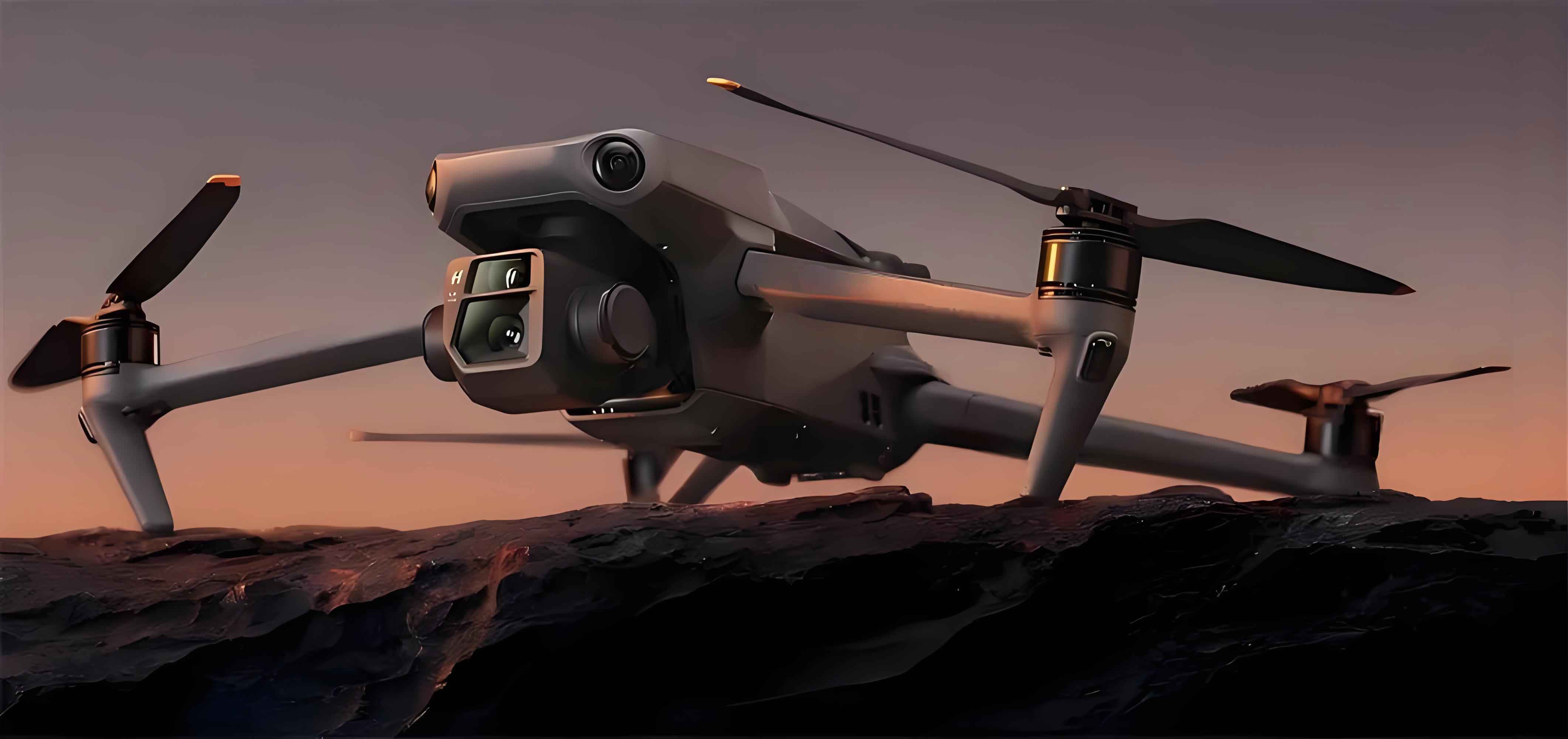
With rapid socioeconomic and technological advancements, surveying accuracy requirements across industries have intensified significantly. The integration of low altitude drone technology with aerial photogrammetry has revolutionized data acquisition, enhancing precision and efficiency in geospatial applications. This synergy addresses limitations of traditional methods, particularly in complex terrains and time-sensitive scenarios. Low altitude UAV systems operate below cloud layers, minimizing atmospheric interference while capturing high-resolution imagery through compact digital cameras and specialized sensors. These systems typically incorporate aircraft platforms, measurement control systems, information transmission modules, and comprehensive support technologies to ensure operational robustness.
The fundamental equation governing photogrammetric accuracy is expressed through the collinearity condition, where image coordinates \((x, y)\) relate to ground coordinates \((X, Y, Z)\):
$$ \begin{bmatrix} x \\ y \\ -f \end{bmatrix} = \lambda \mathbf{R} \begin{bmatrix} X – X_0 \\ Y – Y_0 \\ Z – Z_0 \end{bmatrix} $$
where \(f\) represents focal length, \(\mathbf{R}\) the rotation matrix, \((X_0, Y_0, Z_0)\) the perspective center position, and \(\lambda\) a scale factor. This mathematical foundation enables low altitude drone systems to achieve sub-decimeter accuracy in optimal conditions.
Technical Advantages of Low Altitude UAV Photogrammetry
Comparative analysis reveals significant improvements over conventional surveying methods:
| Parameter | Traditional Surveying | Low Altitude UAV |
|---|---|---|
| Positional Accuracy | 0.1-0.5m | 0.02-0.1m |
| Data Acquisition Rate | 0.5-2 km²/day | 5-20 km²/day |
| Operating Altitude | 500m+ (manned aircraft) | 50-300m |
| Cloud Tolerance | <50% cloud cover | <80% cloud cover |
| Cost per km² | $800-$2000 | $150-$500 |
Four core advantages distinguish this technology:
1. Enhanced Measurement Precision: Operating at 50-300m altitudes, low altitude UAVs capture ground sample distances (GSD) defined by:
$$ GSD = \frac{H \times \text{pixel size}}{f} $$
where \(H\) is flight height and \(f\) is focal length. At 100m altitude with 35mm lens and 20μm pixels, GSD reaches 5.7cm, enabling sub-centimeter feature detection. The technology maintains relative accuracy of 1-3×GSD and absolute accuracy of 3-5×GSD through direct georeferencing.
2. Operational Flexibility: Fixed-wing low altitude drones achieve 60-120 minute endurance with cruise velocities of 60-80 km/h. Multi-rotor systems offer vertical take-off/landing capabilities in constrained spaces. Wind resistance follows the aerodynamic equation:
$$ V_{\text{max}} = \sqrt{\frac{2W}{\rho C_L S}} $$
where \(W\) is weight, \(\rho\) air density, \(C_L\) lift coefficient, and \(S\) wing area. Modern systems withstand 10-15 m/s winds while maintaining stability.
3. Economic Efficiency: Cost reduction manifests through labor optimization and equipment minimization. Traditional topographic surveys require 3-5 personnel covering 1-2 hectares daily, while low altitude UAV teams (2 operators) cover 10-30 hectares daily. The cost-benefit ratio is expressed as:
$$ CBR = \frac{C_{\text{traditional}} – C_{\text{UAV}}}{C_{\text{traditional}}} \times 100\% $$
yielding typical savings of 60-80% for projects exceeding 5km².
4. Application Versatility: Integration with infrared sensors enables thermal mapping through the Stefan-Boltzmann adaptation:
$$ Q = \epsilon \sigma T^4 $$
where \(Q\) is radiant power, \(\epsilon\) emissivity, \(\sigma\) the constant, and \(T\) absolute temperature. This facilitates environmental monitoring, infrastructure inspection, and disaster response.
Field-Specific Implementation Analysis
Land Resource Monitoring
Low altitude drones detect unauthorized land use changes through temporal analysis. Change detection accuracy follows:
$$ A_{\text{detection}} = 1 – \frac{\sum |P_{\text{actual}} – P_{\text{detected}}|}{\sum P_{\text{actual}}} $$
achieving >95% accuracy in identifying construction encroachment and mining activities. Update cycles reduced from quarterly (satellite) to weekly.
Environmental Surveillance
Pollutant dispersion modeling employs Gaussian plume adaptation:
$$ C(x,y,z) = \frac{Q}{2\pi u \sigma_y \sigma_z} \exp\left(-\frac{y^2}{2\sigma_y^2}\right) \exp\left(-\frac{(z-H)^2}{2\sigma_z^2}\right) $$
where \(C\) is concentration, \(Q\) emission rate, \(u\) wind speed, and \(\sigma\) dispersion parameters. Low altitude UAV systems validate models with in-situ measurements at multiple altitudes.
Urban Greenery Assessment
Vegetation indices calculated from multispectral data:
$$ \text{NDVI} = \frac{\text{NIR} – \text{Red}}{\text{NIR} + \text{Red}} $$
enable precise quantification of green space distribution. Shadow reduction algorithms minimize building interference:
$$ I_{\text{corr}} = I_{\text{orig}} \times \frac{\overline{I}_{\text{sunlit}}}{\overline{I}_{\text{shadow}}} $$
improving canopy cover estimation accuracy to ±3% compared to ground truth.
Emergency Response
Disaster assessment timelines compressed through automated damage detection:
| Disaster Type | Traditional Assessment | UAV Response | Time Reduction |
|---|---|---|---|
| Floods | 24-72 hours | 2-4 hours | 92-95% |
| Earthquakes | 48-96 hours | 4-8 hours | 90-92% |
| Landslides | 24-48 hours | 3-6 hours | 87-90% |
Volume calculations for debris flows utilize digital elevation model differencing:
$$ V = \sum_{i=1}^{n} (Z_{\text{pre}} – Z_{\text{post}}) \times \text{pixel area} $$
Additional Applications
Corridor mapping for pipelines and highways employs specialized flight patterns with forward overlap exceeding 80% and side overlap >60%. Agricultural monitoring utilizes crop height models:
$$ \text{CHM} = \text{DSM} – \text{DTM} $$
with biomass estimation accuracy exceeding 85% when calibrated with ground samples.
Operational Workflow
Flight Path Design
Mission planning incorporates terrain-adaptive parameters:
$$ H_{\text{flight}} = \frac{\text{GSD} \times f}{p} + \Delta H_{\text{terrain}} $$
where \(p\) is pixel size and \(\Delta H_{\text{terrain}}\) accounts for elevation variations. Overlap optimization follows:
$$ \text{Longitudinal overlap} = \left(1 – \frac{d}{L_x}\right) \times 100\% $$
$$ \text{Lateral overlap} = \left(1 – \frac{w}{L_y}\right) \times 100\% $$
with \(d\) = distance between exposures, \(w\) = distance between lines, \(L\) = image dimensions.
Ground Control Points (GCPs)
Optimal GCP distribution follows the formula:
$$ N_{\text{GCP}} = 3 + \frac{A}{500} $$
where \(A\) is area in hectares. For 100ha projects, 23 GCPs provide <0.1% relative error. Positioning accuracy follows:
$$ \sigma_{\text{total}} = \sqrt{\sigma_{\text{GNSS}}^2 + \sigma_{\text{target}}^2 + \sigma_{\text{measure}}^2} $$
with modern RTK systems achieving σtotal < 1.5cm.
Aerial Triangulation
Bundle adjustment minimizes reprojection error:
$$ \min \sum_{i=1}^{n} \sum_{j=1}^{m} v_{ij}^T \Sigma_{ij}^{-1} v_{ij} $$
where \(v_{ij}\) is residual vector and \(\Sigma\) covariance matrix. Automatic tie point extraction algorithms process >500 points/image with sub-pixel accuracy.
Image Processing
Dense point cloud generation utilizes semi-global matching:
$$ E(D) = \sum_{p} C(p, D_p) + \sum_{q \in N_p} P_1 T[|D_p – D_q| = 1] + \sum_{q \in N_p} P_2 T[|D_p – D_q| > 1] $$
where \(D\) is disparity, \(C\) matching cost, \(T\) indicator function, and \(P_1\), \(P_2\) penalties. Modern processors achieve 50-100 points/m² density for areas <10km².
Topographic Mapping
Feature extraction employs rule-based classification:
$$ P(\text{class}|f) = \prod_{i=1}^{n} P(f_i|\text{class}) $$
with geometric accuracy validated through:
$$ RMSE = \sqrt{\frac{\sum_{i=1}^{n} (x_{\text{map}} – x_{\text{check}})^2}{n}} $$
maintaining compliance with ASPRS Class 1 standards (RMSE < 10cm) at 1:500 scale.
Conclusion
Low altitude UAV photogrammetry has transformed geospatial data acquisition through its synergistic combination of accessibility, precision, and operational efficiency. The technology’s adaptability across diverse sectors—from precision agriculture to disaster management—demonstrates its fundamental role in contemporary geomatics. Continuous advancements in sensor miniaturization, processing algorithms, and regulatory frameworks will further expand the operational envelope of low altitude drone systems. Future developments will likely focus on enhanced autonomy through AI-driven flight planning and real-time onboard processing, solidifying these systems as indispensable tools in the geospatial professional’s arsenal. The integration of multi-sensor payloads and improved battery technologies will enable more complex missions with reduced operational footprints, ultimately democratizing high-accuracy mapping capabilities across global markets.